Spot-crossing events

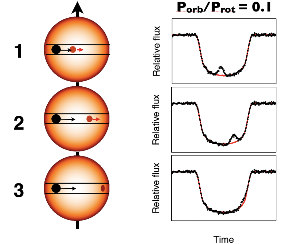
The so-called "spot-crossing events" happen when a transiting planet occults a star spot which is cooler hence darker than the averaged photosphere (see below). This results in a temporary increase of the observed flux. If unaccounted for, the spot-crossing events could be a nuisance, biasing the inferred transit parameters and corresponding planetary properties. However, it was later realized that spot-crossing events can be used to infer stellar obliquity, the angle between the star's rotation axis and the planet's orbital planet. Stellar obliquity in turn can tell us about the dynamical history of the planetary system.

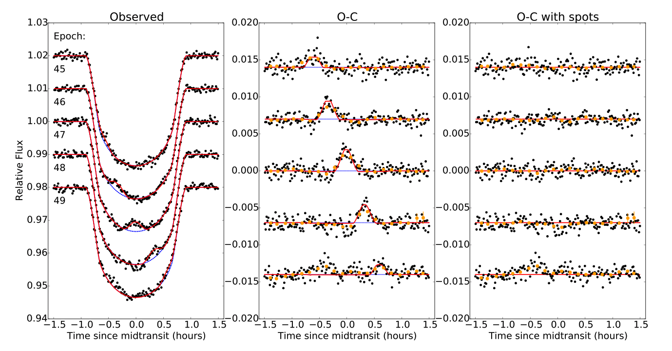
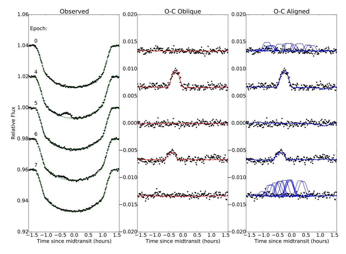
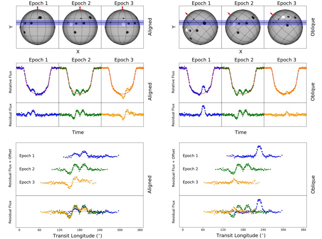
The basic idea of inferring stellar obliquity is simple. In a well-aligned (low-obliquity) geometry, the transit chord of a planet largely overlaps with the trajectory of a crossed star spot. This alignment allows the planet to occult the same spot over multiple transits. The recurrence of spot-crossing events in the observed light curve hence reveals a low stellar obliquity. A prime example is Qatar-2b, a 1.34-day hot Jupiter around a K dwarf. Recent K2 observation in the short-cadence mode unveiled dozens of spot-crossing anomalies. By modeling the recurring spot-crossing events in five consecutive transits, we ( Dai et al 2017) showed that the system has a stellar obliquity less than 10 deg. Esposito et al (2017) later confirmed the low obliquity (λ = 0 ± 10 deg) with Rossiter-McLaughlin measurement from HARPS-N.

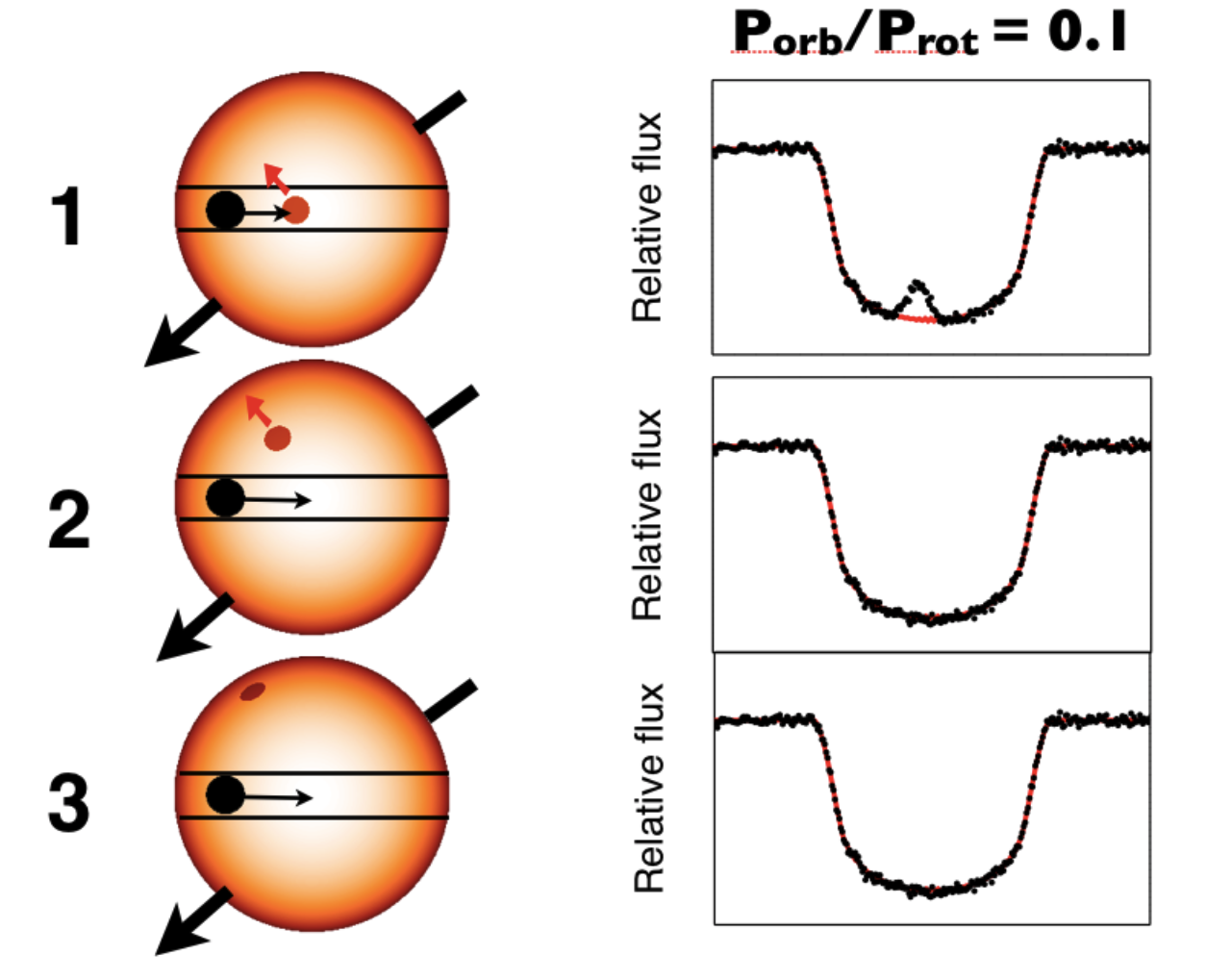
Left: The recurrence of spot-crossing events indicate a low stellar obliquity. Right: A example is Qatar-2b, a 1.34-day hot Jupiter on a well-aligned orbit around a K dwarf ( Dai et al 2017).

Conversely, if spot-crossing events did not recur as expected. one can put a lower limit on the stellar obliquity. Provided that spots last long enough, the absence of additional spot-crossing events implies a minimum obliquity such that the transit chord misses the star spot. This seems to be the case for WASP-107b, a super-Neptune (M = 0.12 Jupiter mass, a/Rs =18.2) around a K dwarf. The short-cadence K2 light curve of WASP-107 showed three isolated clear spot-crossing events. These spot-crossing events did not recur in neighboring transits as would be expected for a low-obliquity geometry. With a Monte-Carlo simulation, we ( Dai et al 2017) demonstrated that WASP-107 has a high obliquity in the range of 40-140˚. The high obliquity has been confirmed by Rossiter-McLaughlin measurement (Triaud et al, in prep). WASP-107 may be a member of the recently discovered "hoptunes" ( Dong et al 2018) i.e. singly-transiting, Neptune-sized or super-Neptune planets. Indeed many of these hoptunes (WASP-107b, HAT-P-11b, Kepler-63b) appear to be misaligned with their host stars, a phenomenon often seen for their bigger brothers: hot Jupiters. The striking similarities between the two groups may hint at a common dynamical origin.

Left: If spot-crossing events did not recur in neighboring transits, the system likely has a high stellar obliquity. Right: This seems to be the case for WASP-107b, a Neptune-mass planet (M = 0.12 Jupiter mass, a/Rs =18.2) around a K dwarf ( Dai et al 2017).

Transit Chord Correlation

In Dai et al 2018, we moved from parameteric modeling of spot-crossing events presented above to a more general and more efficient statistical method which we call Transit Chord Correlation.

The basic idea is still the same. Given a transiting planet with a stellar obliquity close to 0, the trajectory of the planet in the plane of the sky roughly traces out a line of constant stellar latitude on the photosphere (Top panel). If there are active regions (spots/faculae) present on this latitude, they will produce systematic changes in the transit light curves because the active regions tend to have a different brightness than the average photosphere. Darker/brighter features respectively produce increases/decreases in the observed flux (Middle panel). Assuming the active regions last long enough (several orbital periods), a low-obliquity transiting planet will occult the same stellar latitude and the same set of active regions repeatedly. In the bottom panel, we have transformed the light curve from a function of time to a function of stellar longitude. A coherent pattern produced by the underlying active regions emerged which serves as a proxy for low stellar obliquity. On the other hand, for a high-obliquity orbit shown on the right here. The active regions quickly rotate out of the transit chord. Any patterns in the residual flux are produced by different active regions. Therefore, there will be no correlation in neighboring transits.

We applied this method to a few dozens of CoRoT, Kepler and K2 transiting planets with the highest signal-to-noise ratio light curves. We found 10 planetary systems which most likely have a well-aligned orbit as indicated by the strong correlation. Owing to their deep and frequent transits, all of the detected low-obliquity planetary systems are hot Jupiters. Notably, Kepler-45 is only the second M dwarf with an obliquity measurement. The traditional Rossiter McLaughlin method has not had much success with M dwarf because of their higher stellar variability, slower stellar rotation, and fainter optical magnitudes. We also applied the method to about 30 eclipsing binaries, and we found 8 systems that likely have well-aligned orbits.

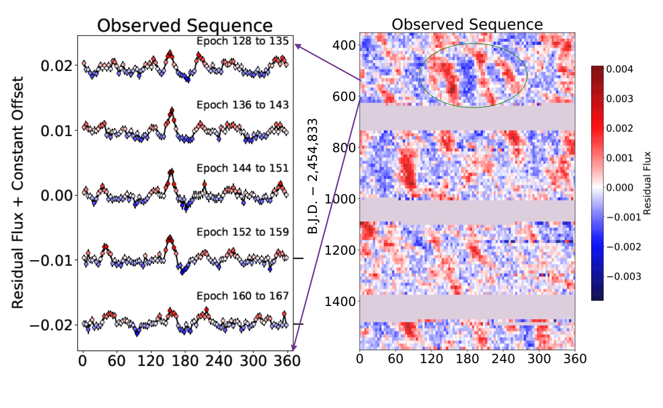
Once a low obliquity is confirmed for a system, i.e. the planet probes a particular stellar latitude repeatedly. One can then reverse the argument. By analyzing their photometric signatures of the active regions, we can study the typical lifetime, spatial distribution, and migration of active regions on the host stars. The figure below illustrates the surface magnetic activity of Kepler-17 as revealed by its planet.

Left—the residual flux of Kepler-17b as a function of the stellar longitude for a series of consecutive transits c.f. the bottom panel of the previous figure. Visually, we can already see a repeating pattern in the residual flux betraying a well-aligned system geometry Right —The same data as the left panel but shown as a heat map. We color code the residual flux such that positive/negative residuals are shown in red/blue. We associate the clustering of positive and negative residuals with the active regions on the host star. The pattern unveils the typical lifetime, size, spatial distribution, and average intensity of active regions. For Kepler-17, the active regions typically span tens of degrees in longitude and they last for 100-200 days before either disappearing or leaving the latitudes probed by the planet. The intensity of the active region changes gradually over time instead of suddenly bursting into existence with maximum intensity. The active regions remain relatively stationary in longitude, with a slight propensity of prograde migration (longitude increases over time). Given the impact parameter b is about 0.27, the stellar latitude near 16˚ seems to be active.

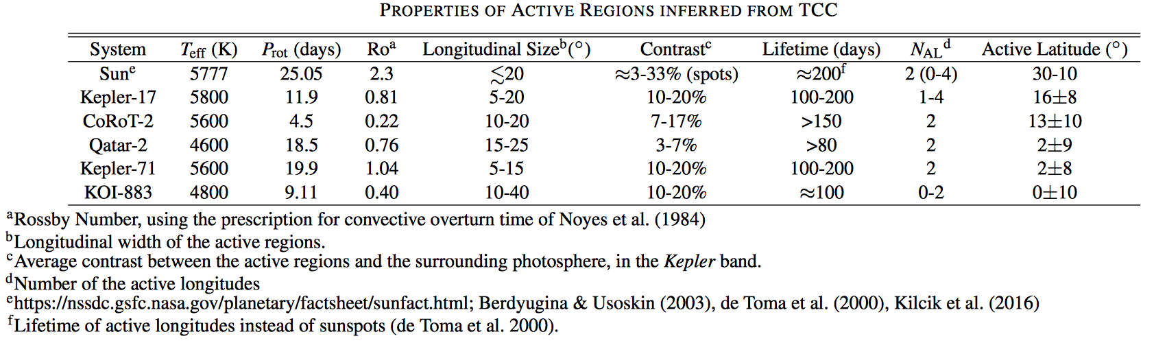
We summarize and compare the properties of the active regions of a few planet hosts with the highest SNR. The Sun is also shown for comparison. Listed in this table are several key properties of stellar activity such as rotation period, size and lifetime of active regions, the active latitude. In many respects, the active regions of these planet hosts are quite similar to our Sun. Measurements of this nature will serve as useful constraints for stellar dynamo theories.