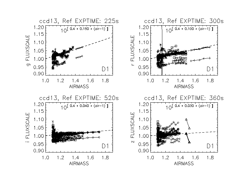
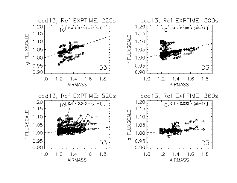
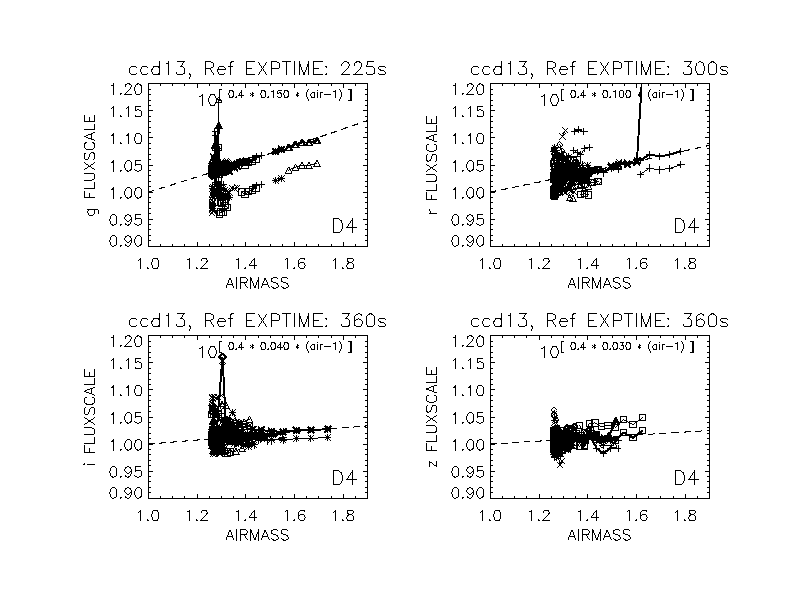
Bottom Line the CFHT Airmass Coeff's - The slope of the data in the airmass versus fluxscale plots agrees with the expected slope using the CFHT canonical value. There are significant offsets between different contiguous image sequences that must be due to transparancy variations between sequences. There are also individual sequences that depart significantly from the expected airmass curve. This must be due to tranparency variations on the given night, indicating it was non-photometric.
Observations - All are CFHTLS Deep observations that have been used in the final photometry. In order to derive this photometry the images must be flux scaled to a reference image. A set of isolated, good S/N objects culled from a SExtractor object catalog is used to calculate the flux scale. Typically hundreds of objects are used and the fluxscale value for a given observation is determined to better than 1%. Observations for a given filter on a given night are taken in dithered sequences of 3 to 7 images. Weather and other considerations provide a real range of 1 to 7 images for the sequences analyzed here.
Analysis - Plotting this fluxscale versus airmass should reveal the trend in fluxscale with airmass. This trend can then be compared to the canonical CFHT airmass coefficient for the given filter to verify the correctness of the value. A first attempt at this revealed a significant scatter in the offsets from sequence to sequence and revealed sequences that were clearly non-photometric, departing from the slope indicated by the canonical airmass coefficient. Photometric nights should have the correct slope, but may suffer from a transparency offset. To correct for this I calculated an offset to the canonical airmass curve for the first observation in a sequence. After applying this offset to all observations in the sequence, it became obvious that the subsequent trend in fluxscale with airmass was following the canonical curve.
Plots -
Below I've made a series of four plots for each of the Deep fields, D1, D3
and D4, one for each of the filters, g', r', i' and z'. Each sequence is
plotted with the same symbol and connected with a line. The bolder points
and lines have had the offset applied to put the first observation in the
sequence on the canonical (dashed) line. The less bold points and lines
have not had this offset applied to show the original distribution.
| D1 | |
| D3 | |
| D4 | |