4. Efficiency

It is important to calculate the efficiency of the final spectral extraction from the SEDM pipeline. This is done by comparing the expected standard star flux with the observed standard star flux. Although that sounds easy, in practice there are many pitfalls to this calculation. This page documents the process by which we derive the efficiency.

At this time it is important to acknowledge the efforts of Jason Fucik, Rich Dekany, and David Hover in producing the models of the SEDM optical system and in performing lab measurements and analysis. In particular, Jason made the crucial discovery of the low throughput ‘smoking gun’ and is leading the acquisition of an improved micro-lens array.

4.1. Standard Flux

The reference data used for this calculation is a tabulated list of fluxes for a given standard star. In our case these are in units of $F_{\lambda ,ref}=erg{s}^{-1}c{m}^{-2}{A}^{-1}$. Since CCDs measure the number of photons observed, our first task is to convert this energy flux into photon ($e^{-}$) flux, $F_{ph,ref}=e^{-}{s}^{-1}c{m}^{-2}{A}^{-1}$.

We know the energy of a photon is $E_{ph}(\lambda )=hc/\lambda erg/e^{-}$. The wavelength dependency must be accounted for when converting to photon flux. Planck’s constant is $h=6.62606885\times {10}^{-27}ergs$ which, when multiplied by the speed of light in $A{s}^{-1}$ gives $hc=1.98782\times {10}^{-8}ergA$. Thus, we get a conversion to photon flux of $F_{ph,ref}=\frac{F_{\lambda ,ref}}{E_{ph}(\lambda )}=\frac{erg{s}^{-1}c{m}^{-2}{A}^{-1}{e}^{-}}{1.98782\times {10}^{-8}ergA}\lambda A$. This gives a final conversion of $F_{ph,ref}=5.034\times {10}^7{F}_{\lambda ,ref}\lambda$, in units of $e^{-}{s}^{-1}c{m}^{-2}{A}^{-1}$.

4.2. Observed Flux

While the previous calculation is pretty basic, calculating the observed spectrum is where many pitfalls are encountered. In particular, since our standard flux is now in $e^{-}{s}^{-1}c{m}^{-2}{A}^{-1}$ and it is very unlikely that the native wavelength bins of our observations are all 1 Angstrom wide, we must carefully account for the native size of the wavelength sampling. To do this, we must use the wavelength scale that is most representative of the cube’s geometry solution.

It is also important that we collect as much of the standard star’s light from the raw image as possible. This means using a large number of spaxels, which makes our calculation more susceptible to background problems. Because of this, we derive our fiducial wavelength scale from the central five arcseconds of the IFU field of view. This avoids any edge effects and should represent the region where most of the standard stars are observed.

In addition, all observations of standard stars are corrected for atmospheric extinction using the standard extinction curves for Palomar (Hayes & Latham 1975).

4.2.1. Wavelength Bins

The new pysedm pipeline uses a linearized wavelength scale. Thus, our observed flux is $F_{ph,obs}=e^{-}{s}^{-1}\mathrm{\Delta }\lambda (\lambda {)}^{-1}$, where $\mathrm{\Delta }\lambda (\lambda )$ is given by the size of the wavelength bins.

4.3. Effective Area

Now we can calculate the effective area of our instrument using the following formula: $A_{inst,eff}(\lambda )=F_{ph,obs}/(F_{ph,ref}\mathrm{\Delta }\lambda (\lambda ))$. All units cancel (see previous formulae) except $c{m}^2$, giving what is called the effective area of the instrument as a function of wavelength.

4.4. Efficiency Ratio

We can now compare this area to the actual area of the telescope, corrected for reflective losses to derive the efficiency, using this formula: $T_{inst}(\lambda )=A_{inst,eff}(\lambda )/A_{tel,eff}$.

For reflective losses of the P60 telescope, we have two mirrors, the primary and secondary, that contribute. If we assume an average of 91% reflectivity for the primary (from reflectometer measurements after the September 2017 re-aluminization) and somewhat less for the secondary which has not yet been re-aluminized, say 90%, we get the total reflective throughput of 82%. We then use the area of the primary mirror, accounting for the secondary obstruction, or $A_{tel}=18,000c{m}^2$. Multiplying the reflective througput times the telescope area gives a telescope effective area of $A_{tel,eff}=14,742c{m}^2$. This is what we divide our instrumental effective area curve by to get the instrumental throughput.

Below is the figure that shows a typical efficiency curve using our best understanding of the calculation and of the instrumental wavelength bins. The efficiency is only as good as the quality of the night and represents an approximation of the true efficiency. Clouds will tend to lower the measured efficiency, but moonlight or other sources of anomolous background will tend to raise the measured efficiency. In general, clouds are a more common source of efficiency offset and so most measurements are lower limits on the true efficiency.

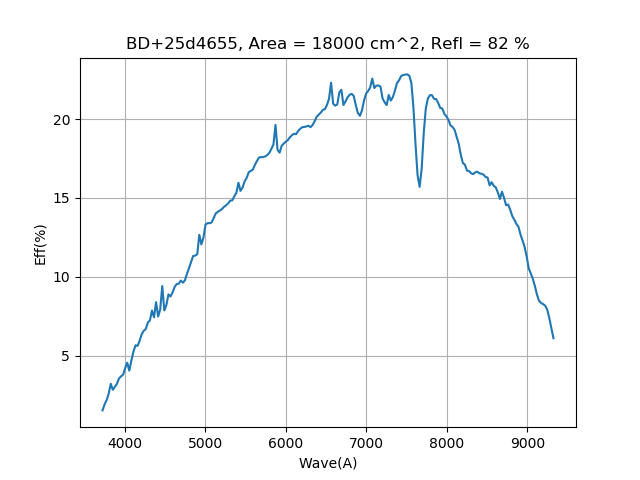
Typical SEDM efficiency curve from 2020 Jan. 01 using BD+25d4655.

4.5. Ray Tracing and Lab Measurements

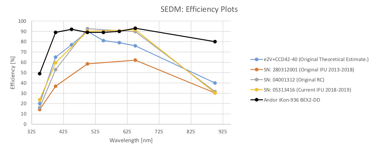
While the SEDM was in the lab, from March through August 2017, we were able to do some analysis of the instrument using a monochrometer and to analyze a ZMAX model of the optics. Below is a figure showing some of the results that we can compare with our on-sky measurements.

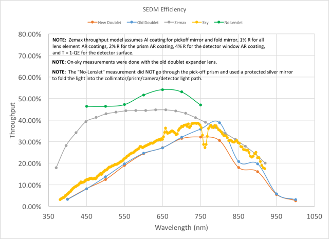
Lab measurements of SEDM throughput (red, blue) compared with the ray-traced throughput for a single spaxel (gray), the on-sky throughput measured without accounting correctly for wavelength bin size (yellow), and the throughput of the instrument without the lenslet array (green).

The yellow curve was derived using the KPY pipeline using incorrect wavelenth bins and is superceded by figure one. We point out that the gray curve is calculated for a single spaxel ray and does not account for losses due to the lenslet filling factor or dead zones between lenses. It is puzzling that our initial (and incorrect) calculation agrees so well with the lab throughput measurements shown by the red and blue curves. It is possible that there is still some accounting for wavelength bins in the lab measurements that needs to be done.

4.6. The Effect of Filling Factor on Efficiency

In our efforts to understand the throughput of the current SEDM, we have tried to estimate the filling factor of the multi-lens array (MLA). In the manufacturing process for any MLA, a certain fraction of the array becomes unusable because of dead zones at the borders of the lenslets. In our analysis, we have found that it is crucial to keep these dead zones as small as possible because, not only do they represent a loss of light, but they are also a source of scattered light. The specification for the orignal MLA was to have a filling factor of around 95%. Our investigations have revealed that, due to a misalignment of the front and back lenses in the MLA, the effective filling factor is actually closer to 80%.

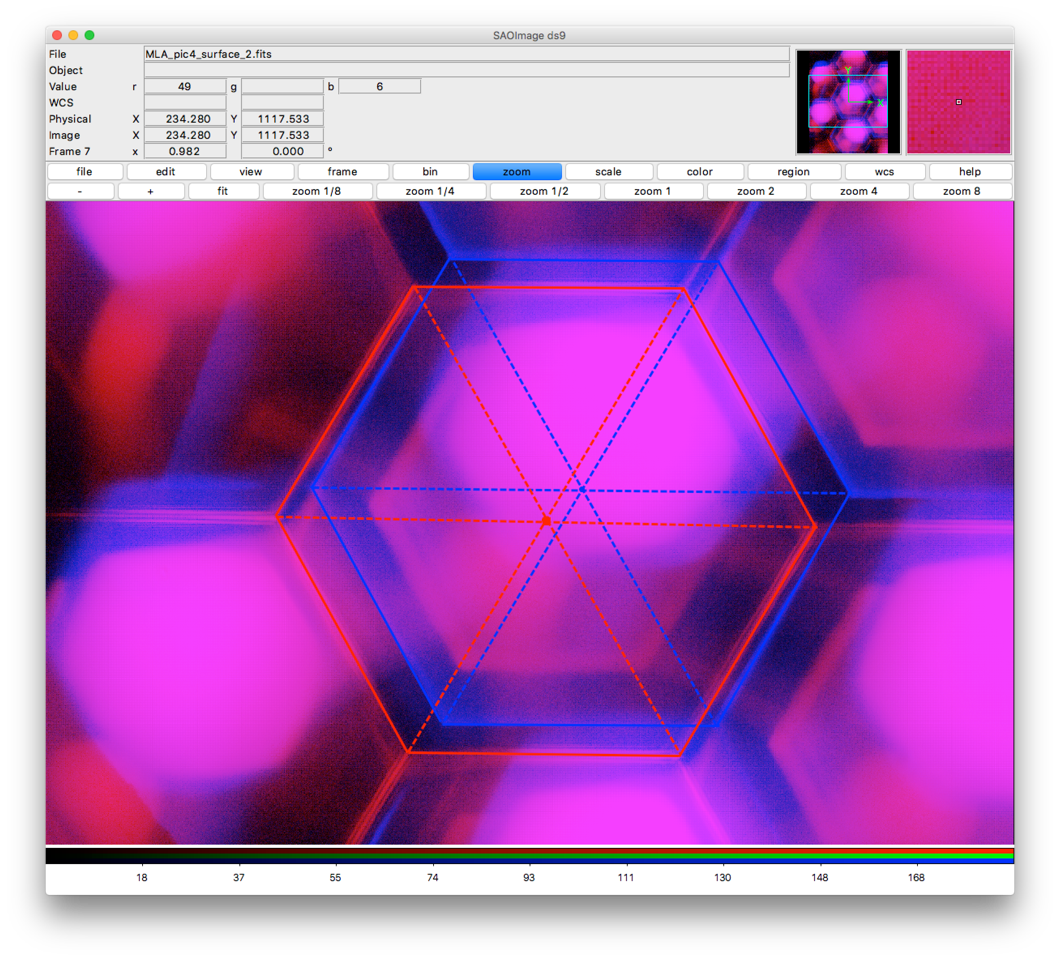
Microscopic view of the SEDM MLA with the red color being the front surface and the blue color being the back surface. The dead zones are apparent as the dark areas and are exacerbated by the obvious mis-alignment of the front and back lenslets.

The impact of this low filling factor is rather extreme and may completely explain the low instrumental throughput. The filling factor enters the throughput calculation as a factor to the power of the number of spaxels involved, $T_{inst}=T_{spax}\times f_{fill}^{N_{spax}}$. Using the peak throughput predicted for a single spaxel (the grey curve in the lab measures figure) of 45%, a filling factor of 80%, and assuming we cover seven spaxels, we get $T_{inst}=0.45\times {0.80}^7=0.09$, which is very close to the measured throughput peak in the figure above of our best efficiency calculation. The remaining difference is likely due to the fact that our standard stars usually cover more than seven spaxels and thus the impact of the filling factor would be greater.

The impact of filling factor is also illustrated by the figure below.

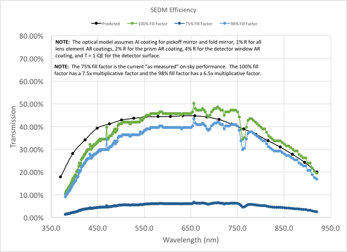
The impact of various filling factors on the efficiency curve. The black curve is the predicted throughput based on the ZMAX model, while the other colors represent different filling factors as indicated in the figure legend.

4.7. The Effect of CCD QE on Efficiency

We also discovered that the original IFU CCD has a 30% lower QE than the more modern CCDs.

The original IFU CCD was apparently an engineering grade CCD. It is now only used as an emergency spare.

4.8. Efficiency Trend

As stated above, the quality of the night most typically reduces the efficiency measurement due to atmospheric extinction (clouds), but can also increase the efficiency if there is a high background (moon). The best way to mitigate these effects is to look at the trend over time. Below is a figure that shows the efficiency in wavlength bins over the course of the last 700 days. This was calculated after re-processing all the archival data with the average fiducial wavelength scale.

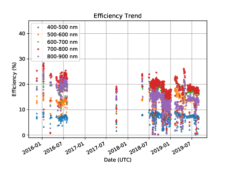
SEDM efficiency in 100 nm bins from 400 to 900 nm for SEDM data that have been reduced using pysedm.

One feature of this plot stands out. There are short periods of higher efficiency that go against the general trend. These are most likely from observations of standard stars that have a high background due to moonlight.

Last updated on 17 May 2023