
|
|

|
CHIMERA Users Manual
The purpose of this document is to describe how to use the CHIMERA instrument for scientific observations. If you're interested in a complete academic discussion of the instruments characteristics please see the CHIMERA instrument paper—CHIMERA: a wide-field, multi-colour, high-speed photometer at the prime focus of the Hale telescope.
Contents
- Quickstart Guide to CHIMERA
- Introduction to CHIMERA
- Starting the CHIMERA Software
- Instrument Operation
- Basic Concepts
- Main Control Panel
- Right Hand Controls
- Camera Synchronization
- Image Naming Control
- Toolbars
- Andor Camera Specific Controls
- Specialized Tools
- FITS image displays
- Target Acquisition and Placement
- CHIMERA GPS Timing
- Ultrafast Observing Mode
- Focusing CHIMERA
- Guiding with CHIMERA
- Conclusions
1. Quickstart Guide to CHIMERA
1.a. CHIMERA Checklist
CHIMERA user interface.
The following is a checklist for getting on-sky and observing with CHIMERA:
- Start CHIMERA RED - start the software for the CHIMERA RED channel on VNC desktop
chimera.palomar.caltech.edu:14using the commandred_chimera. - Start the GPS server - the software will warn you on startup that the GPS server isn't running. Go to the GPS tab on the Advanced GPS panel and first start and then connect to the GSP server. Note that you can have only one instance of the GPS server running at a time and once it's running the CHIMERA BLUE software will automatically connect to it on startup.
- Start CHIMERA BLUE - start the software for the CHIMERA BLUE channel on VNC desktop
chimera.palomar.caltech.edu:15using the commandblue_chimera. - Home the CHIMERA RED filter slide mechanism - use the Mechanisms panel on the Advanced display.
- Home the CHIMERA BLUE filter slide mechanism- use the Mechanisms panel on the Advanced display.
- Home the Dichroic Mechanism - use the Mechanisms panel on the Advanced display on the CHIMERA BLUE GUI. If you're using both channels then insert the dichroic into the field of view.

Initialize and home mechanisms.
- Collect calibration files (i.e. BIAS, FLATS) - to observe biases, make sure that all the lights are off in the dome, set the exposure time to less than 1 millisecond (0.0001). You may wish to collect different BIAS frames for each of the operational modes you intend to use (e.g. conventional vs. EM gain amplifier, different horizontal readout rates, subarrays, etc.)
- Notes on Focusing CHIMERA - The procedure for focusing CHIMERA is a little more complex than a single camera imager since there are two optical channels that must be parfocal. The general procedure is as follows:
- Start by focusing the RED Channel- Set the Birger focus for the RED channel to 9000 to give you adjustment range.
- Select a star on the RED Channel Real Time Display to use for focusing- Place a guide box cursor on the star and focus the red channel using the Autofocus control on the Tools menus of the RED real time diplay. This focuses the transmitted optical beam on the RED channel using the telescope controls
- Select a star on the BLUE Channel Real Time Display to use for focusing- Place a guide box cursor on the star and adjust the BLUE channel focus using the Birger focus control for the BLUE channel.
- Both channels are now parfocal and at best telescope focus.
- Please see this link for more information on focusing CHIMERA.
- Select the amplifer for readout: Conventional and EM gain - If you need exposure times less than 1 second then use the EM amplifier, if exposing longer than 1 second optionally use the conventional amplifier.
- Select the horizontal readout rate (0.1,1.0 conventional, 1.0, 10.0, 20.0, 30.0 EM amplifier) - it is recommended that you use the slowest readout that you can so that you essentially hide the readout using the frame transport process. The faster the horizontal readout rate the higher the noise.
- Do you want to bin the image or only image a subarray? - preset centered subarrays with different binning (up to 4×4) are already configured down to 32×32 pixels. Custom subarray configurations are also supported.
- Determine the number of images per cube? - the maximum size of a FITS cube is 2Gb and the number of images that can be fit in a single cube is determined by the binning and subarray size. Typically you don't want your image cubes to represent more than 5 to 10 minutes of continuous data.
- Check your targeting? Can you identify your target in the Targeting Mode image? - you can position the target in the frame using the Target to Bulls Eye telescope motion control or have the telescope operator move it with the paddles
- Press the Continuous button - the Continuous button makes the system acquire one image cube after the another until the button is turned off
- Press the GO button - the software will continously acqiure one FITS cube after another. It's recommended that you watch the GPS server status during operation if millisecond time accuracy is required.
- Turn OFF Continuous when your observation is complete.
1.b. Retrieving CHIMERA Data
- Retrieving data while at the Observatory - CHIMERA produces a truly immense amount of data during operation. In some observing modes (high speed light curve measurements) the instrument can produce well over 1 million images during a single observing session. It is highly advisable to bring a portable hard drive with you on your observing run so that you can copy the data from the CHIMERA computer prior to leaving the Observatory. Although HPWREN provides a reliable internet link the bandwidth is not infinite and other observers will not appreciate it if you start retrieving terabytes (Tb) of data while they are trying to observe. The best way to retrieve CHIMERA data is to copy it to your portable hard drive before you leave the Observatory.
- Retrieving data from your home institution - you can retrieve your data via
scpdirectly from thechimera.palomar.caltech.educomputer or from a designated proxy (e.g.observer1.palomar.caltech.edu).SSHis generally blocked by the Palomar Observatory firewall except for a designated proxy (observer1.palomar.caltech.edu) that is used for retrieving data. As of this date (Feb 2020) only thechimera.palomar.caltech.educomputer can used for retrieving data via scp. However, the CHIMERA computer will be more tightly integrated into the observing infrastructure in the near future. If you need to remotely retrieve data from CHIMERA please contact the support astronomers for specific details.
1.c. Definition of Terms
There are a few terms used throughout this document that may need a bit of clarification:
FITS Cube - The primary data format for science data produced by CHIMERA. What exactly are FITS cubes? CHIMERA produces FITS cubes (see FITS standard Definition of the Flexible Image Transport System (2016)) where NAXIS=3 with NAXIS1 and NAXIS2 representing the spatial dimentsion and NAXIS3 the image's position in time. The NAXIS3 dimension describes the time series with the first image in the cube representing the earliest time and the last image in the cube the latest time. Each image in the cube (NAXIS1, NAXIS2 representing the image in space) is separated from the next image in time by the exposure time plus any associated readout time. If GPS timing is enabled the FIT header will contain a GPS timestamp for each individual frame.
EM gain amplifier - the CCDs in CHIMERA contain both conventional and EM gain amplifiers that can be used to readout the detector.The EM (Electron Multiplications) amplifiers are described by Andor in the following way: "The Electron Multiplying CCD (EMCCD) operates by amplification (EM Gain) of weak signal events to a signal level that is well clear of the read noise floor of the camera at any readout speed, rendering them single photon sensitive." The EM gain amplifiers work at 1 MHz, 10MHz, 20MHz and 30MHz horizontal readout rates and are particularly useful for low signal levels and / or when exposure times less than 1 second are required.
Conventional amplifier - the "conventional" amplifiers used in the Andor DU888 cameras operate at 0.1MHz and 1.0MHz horizontal readout rates. Conventional CCD amplifiers minimize readout noise by reading the CCD out slowly. The "conventional" amplifiers are used primarily for long exposure times (>= 1 second). When taking long exposures (>= 10 seconds) the minimum noise images are taken using the 0.1MHz readout rate using the conventional amplifier.
2. Introduction to the CHIMERA Instrument
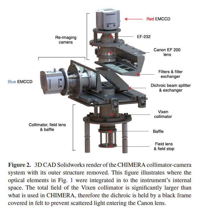
CHIMERA CAD model.
CHIMERA is a dual-channel (red, blue) instrument with 2 filter slide mechanisms and a dichroic mechanism. Each optical channel is equipped with an Andor iXon Ultra 888 EMCCD camera with a 1024×1024 frame transfer CCD. The adjacent diagram displays a 3D CAD Solidworks rendering of the CHIMERA instrument. The dichroic beam splitter transmits light from 570 to 850nm and the reflected light transmits a beam from 300 to 540nm. The light from the transmitted and reflected beams pass through filters mounted in slide mechanisms associated with each channel. The filter slide mechanisms are currently populated by a set of Astrodon Gen2 Sloan filters. In the RED channel the light passed through the dichroic and then through the filter in the slide mechanism. The RED channel slide mechanism is currently populated with Sloan r', i', z' and a custom 600nm filter that is 50nm wide. If only the RED channel is required the dichroic can be removed from the optical path on a slide mechanism similar to the filter mechanism to increase the optical throughput. In the BLUE channel the light from the telescope is reflected by the dichroic and then goes through a filter slide mechanism populated with a Sloan g' and u' filters. The other two positions in the BLUE channel filter mechanism are current not populated.
Each of the optical channels is equipped with a Cannon 200mm f/2 lens which images the collimated beam onto Andor Ultra 888 EMCCD camera for each channel. The commercial Cannon lenses are attached to Birger Electronics remote focus and aperture control mechanism that allow each lens to be controlled by software. The optical beam supplied by the facility Wynne corrector is collimated by a Vixen 380mm f/3.8 commercial lens. The focusing procedure starts with setting the RED channel's Birger focus to 9/10th of its range and then focusing the P200 telescope to produce the best image quality. The BLUE channel is then brought into focus using the Birger focus mechanism to produce parfocal images on both cameras.
The optical design delivers a 5x5 arc-minute field of view to the full frame 1024×1024 format Andor cameras with a plate scale of 0.29 arc-seconds/pixel. Under software control the Andor Ultra 888 cameras can be configured to bin the images up to 16×16 including 2×2, 4×4, 8×8 and 16×16 binning patterns in either dimension (i.e. binned in x and in y). Similarly, the camera support full subarray control by specifiying the starting x and y coordinates of the subarray and then specifying the width and height of the array. A generous collection of predefined subarray configurations such as 1024×1024 binned 2×2 or 512×512 binned 4×4 can be selected at run time.
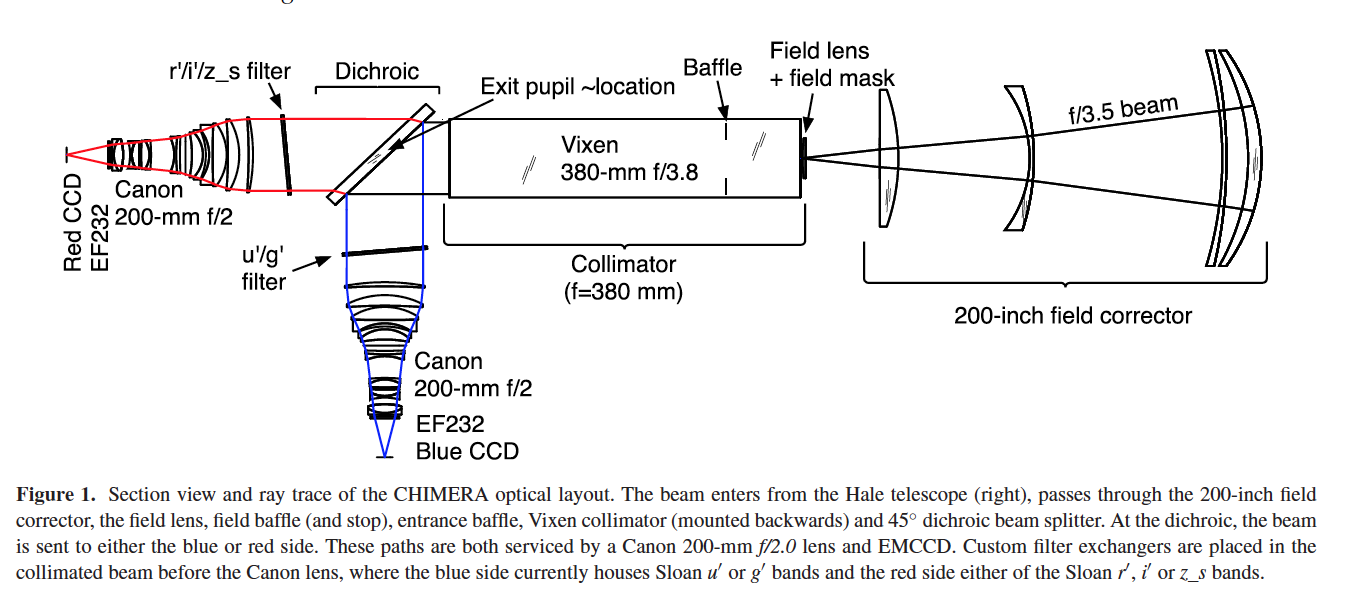
CHIMERA optical design.
2.a. Camera Performance Specifications
The cameras installed in both the RED and BLUE channels of CHIMERA are Andor DU-888 EMCCD's with 1024×1024 sensors with 13×13 micron pixels. The sensitivity and noise of the EMCCD are a direct product of the choice of amplifier (conventional vs. em amplifier) and the horizontal readout rate. The performance specifications for each of the camera are described in the linked PDF files below:
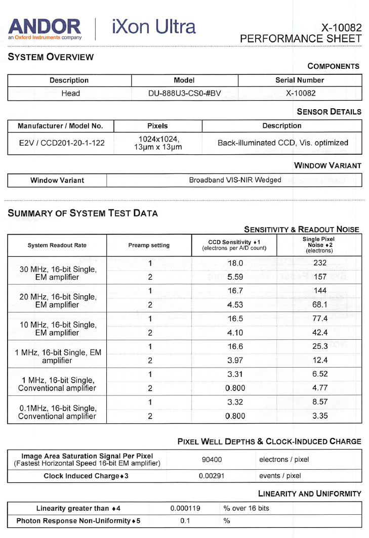
CHIMERA RED Andor DU-888 EMCCD camera performance specifications.
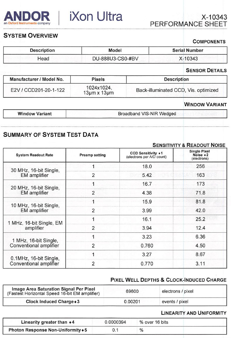
CHIMERA BLUE Andor DU-888 EMCCD
camera performance specifications.
2.b. Software Basics
The CHIMERA software is ultimately derived from a common code-base shared with the DBSP slit-viewing camera and xy offset guider since these instruments using the same Andor Ultra 888 cameras and require many of the same observing features. The software is written in Java and communicates with the Andor cameras using a JNI (Java Native Interface) interface implemented as a shared object library written in C/C++. The C/C++ code relies upon the Andor SDK Version 2 (Software Development Kit) to actually communicate with the cameras over a USB3 interface. Communication with the P200 telescope is via a TCP/IP socket connection and the software automatically maintains separate monitoring and control sockets. Communication with the Birger focus and aperture control mechanisms is via a TCP/IP connection to an RS232 terminal server. The control of the filter and slide mechanism are via TCP/IP connections directly to the ethernet enabled motors that drive each mechanim.
The CHIMERA software consists of two instances of the same program (i.e. red_chimera, blue_chimera) that are started with different command line parameters that trigger different configurations to be implemented at runtime. Each of the program instances connect to specific Andor Ultra 888 cameras based on the camera's serial number. The software is started by opening a terminal window and executing a script that launches each configuration of the program. As of this writing, the CHIMERA computer is located in the prime focus cage adjacent to the instrument to facilitate USB3 connection to the cameras. There are currently plans to relocate the computer to the computer room and communicate with the cameras over a USB3 to fiber interface (i.e. Icron 3022 USB3 to fiber interface). In either case however, the observer never sits at a monitor connected to the instrument computer but relies instead upon VNC desktops hosted by the CHIMERA computer. Typically, one desktop is reserved for each camera and all of the GUI controls are laid out for each camera on the separate desktops. The two VNC desktops are typically numbered chimera.palomar.caltech.edu:14 and chimera.palomar.caltech.edu:15. When the software is started it takes a few moments to establish a connection to the camera and then setup the initial conditions for operation. During this period a warning dialog is displayed asking for you to wait while the camera is configured. The screen will look something like the image below during this period. The GO button doesn't become enabled until the initialization of the camera is complete.
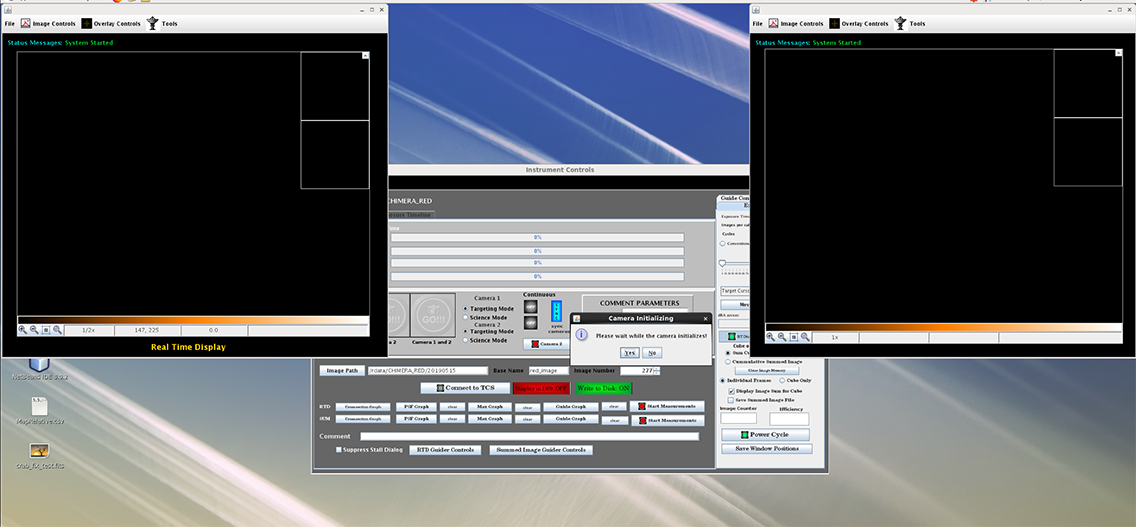
Starting the CHIMERA software.
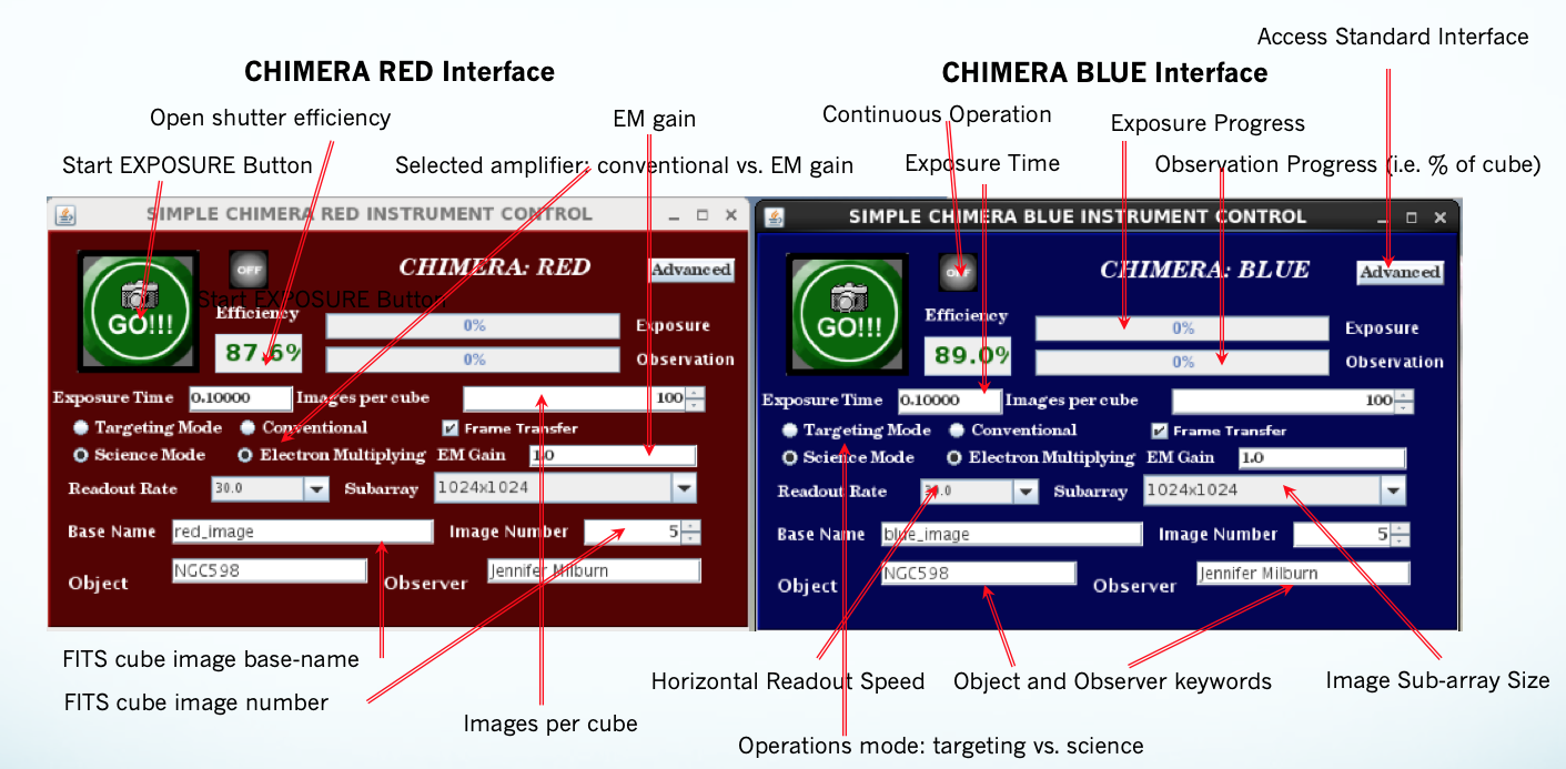
2.c. CHIMERA : The Simple Interface
The full CHIMERA interface can evidently be a little intimidating to novice observers. There are a large number of possible configurations and a lot of tools designed to assist in particular observing scenarios (e.g. guiding) and to assess the image quality during observing. However, there is a subset of the needed controls that are absolutely required to run the instrument and these have been gather together into a "training interface." This interface is presented to the observer when the intrument starts up and the "complete" or "Advanced" interface can be called up by pressing the Advanced button. Let's discuss some of the basic concepts that you need to know.
CHIMERA has 2 operational modes: Targeting and Science: What are these modes used for?
- The Targeting Mode uses the camera as a video camera but numerous parameters can be modified (e.g. exposure time) while the camera is operating in Targeting Mode. When you're in Targeting Mode you are NOT saving data to the hard drive, the images are transitory and cannot be saved. The main purpose of the targeing mode is allow you to setup the image frame so that your object is in the right place and you know the signal that you will receive. You can change the exposure time and the subarray size on the fly and have a good appreciation for how your images will look once you start observing "for real."
- The Science Mode is what you actually use when you're collecting your data. CHIMERA stores images in FITS cubes on disk so before you switch to Science Mode you need to know how many images you want in each cube. There is a limit to the number of images you can store in an image cube and the limit of the exact number of images is determined by the subarray size and binning. Ultimately, you cannot create FITS cubes greater than 2Gb in size. If you try to create a cube that will be greater than 2Gb in size the system will display a dialog warning you that this isn't a good idea (i.e. it will crash the software) and it will set the cube size to the maximum allowed for the selected subarray and binning configuration.
CHIMERA automatically creates a date stamped directory when the software starts if a directory for that date hasn't already been created. The name of the FITS cube is a combination of the Base Name and the Image Number. Both of these parameters can be accessed from training interface. Observers are free to use the combination of Base Name and Image Number in any way they wish. It's fairly typical for an observer to use the object name and the basename with an underscore separating the basename from the image number and then set the image number to one at the start of the observation of a particular object.
The most critical parameters for determining the signal to noise of your observations is the choice between the Conventional and Electron Multiplying amplifiers and the associated horizontal readout rate. In general, the Conventional amplifier is lower noise but the fastest horizontal readout rate is 1 MHz which requires ~ 1 second to readout the full 1024×1024 array. For exposures times of 1 second or longer that readout can effectively be hidden by selecting frame transfer mode and you can achieve open shutter efficiencies of greater than 90%. For exposure times less than 1 second however the Conventional amplifier cannot achieve acceptable open shutter efficiencies. For exposure times less than 1 second the Electron Multiplying amplifier offers alot of advantages. The primary reason that the Electron Multiplying amplifier is more useful when using exposure times less than 1 second is that the horizontal readout speeds for the Electron Multiplying amplifier included 10, 20 and 30 Mhz rates. When combined with frame transfer you can achieve high open shutter efficiencies (i.e >= 90%) using the 100 millisecond exposures using the 10Mhz rate, 50 millisecond exposure using the 20Mhz rate and 33 millisecond exposures uisng the 30Mhz rate.
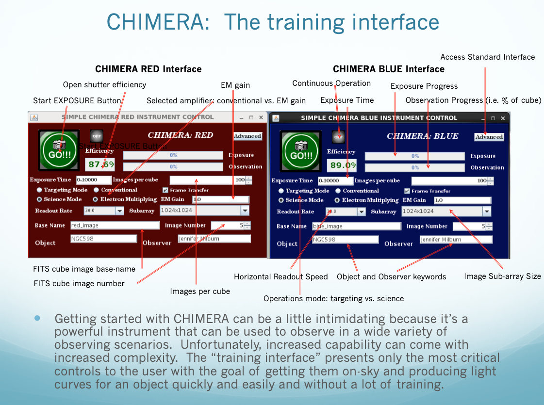
The simple CHIMERA interface.
3. Starting the CHIMERA Software
How do you start CHIMERA and what steps are needed to get the instrument ready for observing?
Connect to the 2 VNC desktops used for each camera: vncviewer chimera.palomar.caltech.edu:14 and :15.
If you need GPS timestamps for each image then start the gps_server program. Start the camera software for one camera on each desktop, it doesn't matter which desktop is used for which camera. The startup command script is red_chimera and blue_chimera. If one or more of the cameras doesn't start (i.e. the GO button doesn't turn green and displays the GO image) try cycling power on the camera or cameras that don't start correctly. The CHIMERA cameras are plugged into a network power switch that can be accessed from the browser on the CHIMERA computer (ask the support astronomers to show you the link on the desktop). The software checks the serial number of the camera it connects to so the system can't get confused about which camera is which.
Once the software is started press the GO button and wait for the image acquisition to start (images will be displayed in both the real time display and the summed image display). It may take an extended period for the first image to arrive so please be patient. Typical delay times for the first image to appear is ~ 30 seconds but it can take well over a minute before the first image is diplayed in some cases. Please be patient and just allow the camera to deliver the first frame when it's available.
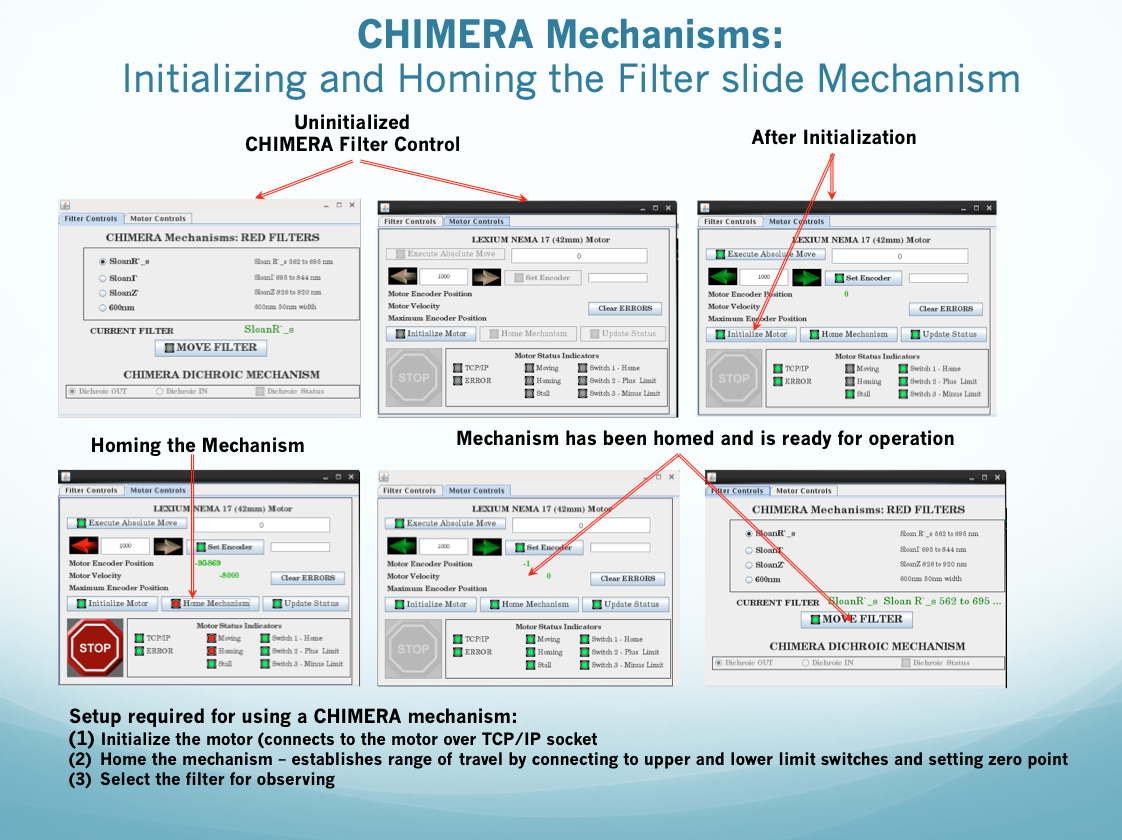
CHIMERA mechanisms.
Open the CHIMERA Filter Mechanism dialog for each camera and perform the following steps to ready the mechanism for operations. First select the Motor Controls tab on the mechanism dialog and then press Initialize Motor and wait for the control icons to turn green. Once the Home button is activated (i.e. icon is green), press Home and wait for the homing sequence to finish, this may take a couple of minutes because the mechanism must determine the limits of the mechanisms range. Once the homing sequence is complete, switch to the Filter Controls tab, select the filter you wish to use by selecting the associated radio button and then press the Move Filter button. The status icon on the Move Filter button will turn red while the move is taking place and then back to green when the move is completed. The filter mechanism is now ready for use and the selected filter is in the optical path. You need to preform this task for each camera since there are separate filter mechanisms for each optical path.
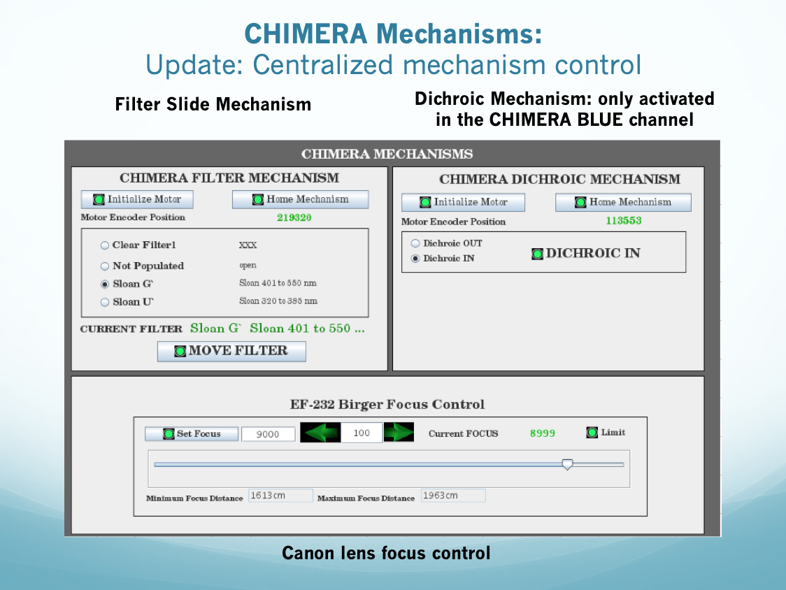
Updated CHIMERA mechanism control.
Using one of the camera interfaces (it now defaults to the BLUE side), select the CHIMERA Dichroic Mechanism control. The convention is to home this mechanism with the blue camera interface since this mechanism enables light to arrive at the blue camera. Select the Motor Controls tab, press the Initialize Motor button followed by the Home button and wait for the homing sequence to complete. After homing the mechanism is moved out of the optical path. If you intend to use the blue camera, select the Filter Controls tab and press the Dichroic IN radio button and wait for the mechanism to move into the optical beam. Once the indicator on the right says DICHROIC IN with a green indicator icon the system is ready for observing with the blue camera.
4 Instrument Operation
4.a. Basic Concepts
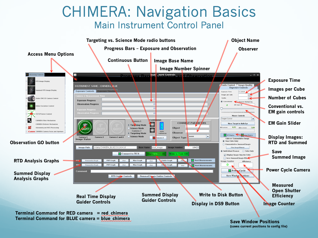
The primary scientific products produced by CHIMERA are FITS image cubes of variable size and format. The instrument operates in two modes: targeting and science mode, controlled by selecting the associated radio buttons on the main instrument control GUI. Images are never saved when the system is in Targeting Mode and to acquire scientific data you need to specify the number of images per cube and select Science Mode operation. The figure below depicts the main instrument control GUI and its associated controls.
Basic instrument control.
When the instrument is in Targeting Mode the camera produces a continuous stream of images delivered at between 1 and 2 Hz to assist the observer in setting up the observation. Targeting mode allows all of the camera operational parameters to be changed and the effect of the change to be immediately displayed to the user (e.g. changing exposure time, readout rate, etc.). There are some limitations on what parameters can be changed however. You cannot change from conventional to em amplifier operation during targeting mode operation; you must first stop taking images, change the amplifier setting and then resume targeting mode operation. The GUI is designed to disable the controls for features that cannot be changed during targeting mode operation when the camera is taking images. The disabled controls become available once image acquisition is stopped. When the camera is in targeting mode the images are never saved.
The acquisition of scientific data is always carried out when the instrument is in Science Mode and the product is always a FITS image cube (NAXIS=3). The instrument was designed to continuously acquire images and write them to FITS image cubes up to 2Gb in size. Typical science operations produce one image cube after another when the instrument is in "continuous" operations mode (see "Continuous" button on the main instrument control GUI) with a minimum of down time between FITS cubes. The objective is to provide a continuous stream of images that are written to disk as fast as the camera can supply the data to the computer. When science mode operations are taking place the color map used in displaying the images within the internal image controls (real time display and summed image control) changes from heat (used during Targeting Mode) to grey scale (used during Science Mode operation). The number of images in the data cubes, and consequently the number of images acquired before resetting and starting a new cube, is controlled by the images in cube spinner control located on both the main instrument controls panel and on the Andor camera controls panel.
Let's go through all of the controls on the Instrument Control panel individually to discuss exactly what each does.
4.b. Main Instrument Control Panel
There are two sets of exposure and observation progress bars in the upper center portion of the instrument controls panel; one for each camera. The second camera exposure and observation progress bars are only activated if the second camera has been connected (i.e. using the Camera 2 button)
- Exposure Progress - displays the progress of the current exposure. The exposure progress bar is only activated when the exposure time is greater than 0.5 seconds (i.e. it doesn't make sense for very short exposures). The exposure progress bar always stops on the last image of a data cube so don't worry that the last image progress doesn't seem to update.
- Observation Progress - displays the progress of the current FITS cube observation. The observation progress bar displays the percentage of the total observation progress. For example is you are observing a 100 image FITS cube and so far the 10th image has just been observed the observation progress will diplay 10%.
4.c. Right Hand Camera Controls Panel
There are two sets of exposure and observation progress bars in the upper center portion of the instrument controls panel; one for each camera. The second camera exposure and observation progress bars are only activated if the second camera has been connected (i.e. using the Camera 2 button).
- Exposure Progress - displays the progress of the current exposure. The exposure progress bar is only activated when the exposure time is greater than 0.5 seconds (i.e. it doesn't make sense for very short exposures). The exposure progress bar always stops on the last image of a data cube so don't worry that the last image progress doesn't seem to update.
- Observation Progress - displays the progress of the current FITS cube observation. The observation progress bar displays the percentage of the total observation progress. For example is you are observing a 100 image FITS cube and so far the 10th image has just been observed the observation progress will diplay10%.
- Exposure Time - this text field contains the exposure time in seconds
- Images per Cube - the number of images to include in a single FITS cube
- Cycles - the number of FITS cubes to acquire (i.e. with a single press of the GO button)
- Conventional and Electron Multiplying gain radio buttons - changes camera amplifier mode from conventional to EM gain amplifier.
- EM Gain controls - you can enter the specific EM gain in the EM gain text field to specify a particular value or you can adjust the gain by moving the slider. The effective EM gain is displayed in green above the EM gain slider. The EM gain has no effect in conventional mode.
- Mouse Controls - the mouse controls combobox can be used to change the selected mouse cursor. The options include the following selections: (1) target cursor, (2) bull-eye cursor, (3) guide box cursor, (4) background box cursor, (5) image calibration cursor (deprecated), (6) no cursor. The mouse controls combobox is linked directly to the real time display and can alternately be accessed using a right mouse click on the real time display image.
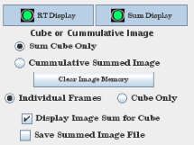
- RT Display and Sum Display buttons - these two buttons control whether images will be displayed during acquisition in the associated image display (i.e. real-time or summed displays). Turning off image display can have a profound effect on the open shutter efficiency if the exposure times are short.
- Cube or Cummulative Image modes - the Sum Cube Only and Cummulative Summed Image radio buttons determine whether the summed image display is cleared after each FITS cube (i.e. Sum Cube Only) or if it continues to accumulate until the Clear Image Memory button is pressed. The Clear Image Memory button can always be used to clear the summed image and reset the summed image display.
- Individual Frames or Cube Only radio buttons - The Individual Frames and Cube Only radio buttons determine whether the summed image display is updated after each image or if it only displays the summed image after the completion of an image cube. These controls are useful if you're using cube only guiding where the summed cube is analyzed for guide correction but individual frames are skipped and not used (except as they are included in the summed image). To configure the system for cube only guiding, select the Cube Only radio button and the Sum Cube Only radio button.
- Display Image Sum for Cube - determines whether to display the summed image after the completion of a FITS cube.
- Save Summed Image File - determines whether the summed image for the FITS cube is saved to disk as a separate file.
- Image Counter - the number of individual images acquired for targeting mode and the number of consecutive FITS cubes during science mode acquisition. The counter is particularly useful when the system is in "continuous" mode as a counter for the number of images taken.
- Measured Open Shutter Efficiency - the percentage of the time during the last image cube that the camera was collecting light. This is basically the ratio of the total exposure time and the measured observation time (i.e. the time from the start of the acquisition until the analysis is complete).
- Power Cycle button - this button shuts down the camera library, power cycles the camera using the network power switch and then reconnects to the camera and initializes all of the system values. In case of a camera lockup (a rare but not unheard of condition) you can often recover by cycling the camera's power. This process can take a couple of minutes to complete and you need to wait until the GO button first disappears and finally reappears.
- Save Window Positions button - this button saves the current position of the instrument control panel and the real time and summed image displays to the configuration file. When the software is restarted the windows should reappear in the same position as when this button is pressed.
4.d. Camera Synchronization
Each of the cameras (RED, BLUE) support an external command channel over TCP/IP. Using the Camera 2 button on either of the instrument control panels you can connect to the other camera channel. The control of the second camera is limited to changing observing modes (i.e. targeting vs. science mode) and starting and stopping an exposure. If you intend to use the camera synchronization functions you should completely setup the desired exposure on the second camera and then start the exposure for both cameras from one instrument control panel. To synchronize the two cameras carryout the following steps.
- Connect to the second camera by pressing the Camera 2 button (note you may need to press it twice the first time to turn the icon green). This establishes a TCP/IP command connection to the other camera. If the icon does not turn green, check the status of the second camera software which must be running. If the connection is successful the GO button for camera 2 is enabled.
- Synchronize the cameras by pressing the SYNC button. The SYNC button turns green in color. When the cameras are synchronized the individual GO buttons for cameras 1 and 2 are disabled and the combined GO button is enabled. Pressing the combined camera 1 and 2 GO button will now start exposures on both cameras. The level of synchronization is within 50 millisecond as the command to start the exposure is communicated to the second camera and the exposure thread is started. The level of synchronization is dependent upon operating systems thread launch and scheduling priorities and either camera can end up being the first to start acquision.
- To disable synchronization simply press the SYNC button and it will return to a blue color and the camera 1 and camera 2 GO buttons will be enabled and the combined GO button will be disabled. If you wish to disconnect completely then press the Camera 2 button and it will have its icon turn red and the Camera 2 GO button will be disabled.

Synchronization of the RED and BLUE cameras.
4.e. Image Naming Conventions and Storage Locations
The software automatically creates an image directory under the base directory with the format YYYYMMDD. Image name are a concatenation of the base name and the image number and both of these can be edited at will. It is impossible to accidently overwrite a FITS image since the software checks to see if the file exists and then adds a _o to the new file name to prevent overwriting. Observers can also control whether files are written to disk and can choose to automatically display images in DS9. The same portion of the instrument control panel also contains a control to toggle connection to the TCS that can be used to reestablish a connection to the TCS in case of a TCS reboot. The object, observer and obstype keyword values in the header can be specified in the Comment Parameters panel.
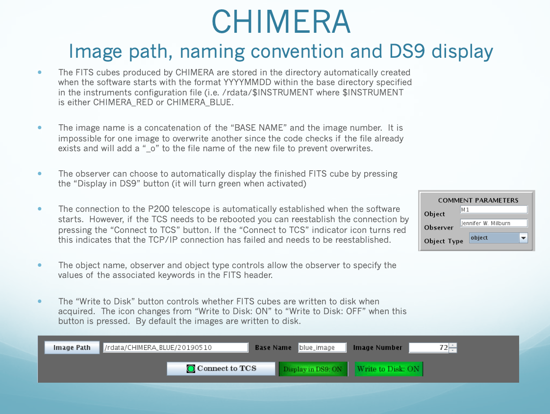
Image naming conventions.
4.f. CHIMERA Toolbar
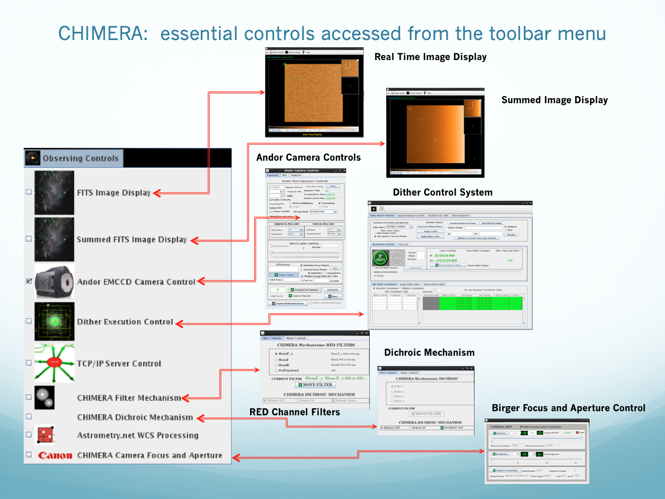
The solar system icon in the upper left corner of the main Instrument Controls panel opens a drop-down menu when pressed that gives the user access to additional instrument controls. The following is a short description of each of the instrument controls avalable from this menu. Selecting and checking a menu item from this drop-down makes the associated control visible on the desktop. By default, the real-time FITS image display and the summed image display are both visible when the software is started while the other controls are hidden.
- FITS Image Display - The FITS Image Display control is the real-time image display system for CHIMERA. Each time an image is acquired from the camera it is displayed in this control.
- Summed FITS Image Display - The Summed FITS Image Display control displays the cummulative sum of the images displayed in the real-time control. Each time an image is acquired it is added to the previous summed image and the summed image is displayed. The Summed Image Display works both with the "targeting" and "science" operational modes but the behavior can be slightly different in each case. For the "targeting" mode the summed image continues to accumulate until the user stops taking images and then it resets and will start accumulating again when the targeting mode begins again. In the case of "science" mode operations the default behavior is to accumulate the sum throughout the collection of an individual FITS cube and then reset at the end of the cube. However, it is possible to change this behavior by selecting the Cummulative Summed Image radio button and the accumulation continues from one FITS cube to the next until the observer manually clears the summed image display buffer by pressing the Clear Image Memory button on the main Instrument Controls panel. The observer can also choose whether to display the summed image after each individual frame is added or to only display the sum of the entire FITS cube when the cube is complete. The Summed Image Display behavior is controlled by the radiobuttons on the main Instrument Controls panel in the right center portion of the control. In either observing mode the summed image memory can be clear by pressing the Clear Image Memory button. Ths summed image for an individual FITS cube can also be written to disk along with the raw FITS cube by checking the Save Summed Image File checkbox. The summed image written to disk has the same basename as the raw FITS cube but with
_summed.fitsappended to the file name. - Andor EMCCD Camera Control - The Andor Camera Controls panel contains all of the controls for manipulating the Andor Ultra 888 EMCCD camera and is described in detail below (see discussion).
- Dither Execution Control - The Dither Control System dialog integrates the camera controls with the telescope control system to allow complex observing patterns to be executed. Dither observations can be as simple as a 5 point rectangular dither pattern with variable scaling to complex maps that observe FITS cubes at over a hundred sky positions. The Dither Control System is explained in detail below.
- TCP/IP Server Control - by default the CHIMERA software automatically starts a TCP/IP server than can be used to synchronize operations between camera. The TCP/IP Server Control allows the observer to start or stop this service and displays a simple log of the commands received on the TCP/IP port and the responses sent to the client.
- CHIMERA Filter Mechanism - the filter slide mechanism has already been discussed in detail in the quick-start section of this manual. Changing filter for the associated slide mechanism is the primary purpose of this control.
- CHIMERA Dichroic Mechanism - the dichroic slide mechanism is used to insert the dichroic into the optical path. By default, the dichroic is removed from the path when the mechanism in initialized and homed. If the BLUE channel will be used for observing the dichroic must be inserted into the optical path or no light from the telescope will reach the BLUE channel camera.
- Astrometry.net WCS Processing - Astrometry.net is an incredibly useful tool for refining the WCS in individual FITS images. This control provides a GUI for Astrometry.net which is installed locally on the
chimera.palomar.caltech.educomputer. This control is useful for the analysis of the summed images if they are written to disk. - Canon CHIMERA Focus and Aperture control - this control provides access to the Birger focus and aperture control mechanism for this camera channel. The Birger Electronics focus and aperture control mechanism for Canon lens is automatically connnected when the software starts and automatically changes the focus to the last known best focus position. Controls include a means to set the focus to any valid value and to incrementally shift focus by a set amount in either direction. Sliders are also available to shift focus and to select among the available apertures. By default the aperture mechanism is always set to the minimum f/2 value when the mechanism is initialized.
Summed image display.
Essential controls.
5. Andor Camera Specific Controls
5.a. Controls GUI
The Andor Camera Controls GUI contains controls that allow the observer to manipulate all aspects of the camera's operations. Let's start by discussing the simplest parameters: the exposure time, the number of images to combine into a FITS cube and the number of cyles of this observation to perform. The exposure time is entered in the Exposure Time (sec) text field and requires a carriage return to propogate the value to the camera. The number of images per cube is represented as a spinner control and specifies the number of images that will be in the FITS image cube collected in a science mode acquisition. The cycles spinner specifies the number of image cubes observed during a single observation. In the image below, the observation that will be carried out is two (cycles=2) FITS cube containing 500 images obtained with an exposure time of 0.025 seconds.
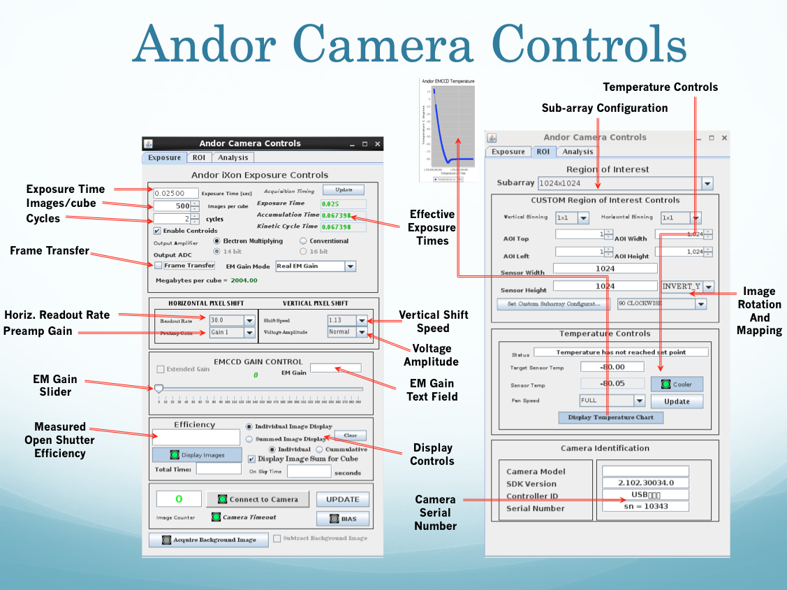
Andor camera controls.
The speed of the imge readout is controlled by a combination of the horizontal shift and the vertical pixel shift speeds. The Conventional and Electron Multiplying gain amplifiers each support a different set of horizontal readout rates. The conventional amplifier supports 1Mhz and 0.1Mhz horizontal readout rates resulting in a total read time for the 1024×1024 detector of 1 second and 10 seconds respectively. The EM gain amplifier support 1Mhz, 10Mhz, 20Mhz and 30Mhz horizontal readout rates and is typically operated in the default 30Mhz mode. The vertical pixel shift speed rarely needs to be adjusted from the default 1.13 value. However when using the 30Mhz horizontal readout you can select the faster 0.6 vertical pixel shift value but the images won't completely transfer (i.e. there will be a shifted frame with a blank section) unless you increase the voltage amplitude.
The following is a list of each control on the Andor Camera Controls panel with a description of the effect of the control on the operation of the camera.
5.b. Exposure Configuration
- Exposure Time - this control sets the actual exposure time. This control requires a carriage return to propogate the exposure time to the camera.
- Images per cube - this spinner sets the number of images to include in the FITS cube.
- Cycles - the number of cycles is effectively the number of FITS cubes to acquire with a single press of the GO button.
- Acquisition Timing: Update - this control queries the camera for the exposure time, accumulation time and kinetic cycle time. The acquisition timing values are displayed in read only text fields below the Update button. When the camera is not in frame transfer mode the exposure time is identical to the requested exposure time in the Exposure Time text field. However, when frame transfer is selected the exposure time may actually be greater than the requested exposure time due to the time required to transfer the image to the frame store and then read it out. The accumulation time is the time required to expose and then readout the array when the system is coadding frames inside the camera. Coadding frames is not currently supported by the CHIMERA software. The kinetic cycle time is the actual time between the start of single exposure and the start of the next exposure including the read time. The kinetic cycle time represents the time between images including the readout time. Note that the effect of frame transfer on the acquisition timing parameters cannot be calculated when the system is in targeting mode. If you need the exact kinetic cycle time before you start a long acquisition you should observe a small image cube (>= 2 images) to allow the system to fully take into account the effect of the frame transfer.
- Output Amplifier radio buttons - The camera can operate in either Conventional or Electron Multiplying gain mode. The mode is controlled by selecting the associated radio button.
- Output ADC: for earlier versions of the Andor EMCCD camera (PCI version) you could choose between 14 bit and 16 bit amplifiers. With the current version of the camera (Andor Ultra 888 EMCCD) only the 16bit version is available so both the 14bit and 16bit radio buttons have been disabled.
- Enable Centroids checkbox - If you wish to evaluate the image quality using the internal guide box controls and plots or implement guiding the Enable Centroids checkbox must be checked. If you are doing extremely high speed acquisition you may be able to increase the open shutter efficiency by disabling the centroid calculations. By default, centroids are enabled.
- Megabytes per cube - Problems can occur if an individual image cube greater than 2Gb in size are observed. How big the requested image cube may be is dependent upon not only the number of frames but the size of the frames based on binning and subarray configuration. Each time you modify one of the parameters that effects image size (i.e. number of frames, subarray size, binning) the megabytes per cube value is calculated and displayed. If you configure the system to create a file greater than 2 Gb a warning dialog will be displayed but it will not keep you from taking the observation.
- EM Gain Mode - The EM gain mode can interpret the applied EM gain in different ways determined by the selection of the EM Gain Mode selection control. The options are: (1) Default 0-255, (2) 0-4095, (3) Linear mode, (4) Real EM Gain mode (Default = Real EM gain mode). It is recommended that you keep the EM gain mode in the default setting. By default, the EM gain is limited to a Real EM gain of 300 to avoid a long term degradation of the detector when values greater than 300 are applied. It is particularly important to keep the EM gain below 300 when the total flux on the detector is high.
- Horizontal Pixel Shift readout rate - For the conventional amplifier the selections are 1Mhz and 0.1Mhz; for the EM amplifier the selections are 1Mhz, 10Mhz, 20Mhz and 30Mhz. The readout time is directly proportional to the horizontal readout rate with the following readout times required for a full frame image:
- Preamp Gain - The preamp gain can be either Gain1, Gain2 and Gain3. Unfortunately, the numeric value of the preamp gains aren't provided by Andor. There is no preference for one value of preamp gain over another.
- Shift Speed - The shift speed combobox controls the time it takes to shift one row of data vertically. Small values indicate higher speed since the vertical shift speed is essentially the amount of time in micro-seconds (μ) it takes to shift one row to the adjacent row. By default the vertical shift speed is set to the second fastest value (1.13). Be aware that when you increase the vertical shift speed (e.g. 0.6 micro-seconds) you may also need to increase the voltage amplitude. With earlier version of the Andor 888 camera you could occassionally run into a setting that failed to completely transfer a frame during readout (e.g. 30Mhz, 0.6 micro-seconds, Normal amplitude). Increasing the voltage amplitude was the cure for this problem. The choices of vertical shift speed are: (1) 0.6, (2) 1.13, (3) 2.2, (4) 4.33 with the default equal to 1.13 micro-seconds.
- Voltage Amplitude - (See shift speed) Possible voltage amplitudes are as follows:
- EM Gain slider and text field - You can control the applied EM gain by moving the slider if the system is in EM gain observation mode. The current EM gain is displayed above the slider in green text. You can also directly enter the requested gain in the EM gain text field to the center right of the control. The EM gain range is from 0 to 300 and currently the choice of extended gain (i.e. > 300) has been disabled to preserve the detector from damage.
- Efficiency: The "open shutter" efficiency is automatically calculated for each FITS cube by measuring the total time the detector was exposing and the actual time required to acquire the cube. For example, in the image of the Andor Camera Control below the "open shutter" efficiency is 97.5% with a total time of 51.0 seconds during which the detector was exposing for 50.0 seconds. The Total Time and On Sky Time are automatically displayed in their associated text boxes. Note that this measurement takes into account all overheads and is an actual measure of the efficiency rather than an estimate. The factors that most commonly influence the open shutter efficiency are the behavior of the image displays and the length of the individual exposures. Let's take the example of using the conventional amplifier with the 1Mhz readout. If you are observing 1.0 second exposures with the 1Mhz horizontal readout rate the read time is ~1.1 seconds and the exposure time is 1.0 seconds requiring a total 2.2 seconds for 1.0 second of on-sky exposure. The resulting efficiency is always less than 50% since the readout time is greater than the exposure time. If we now increase the exposure time to 10 seconds, the open shutter efficiency is now greater than 90% since the exposure is a factor of 10 greater than the readout time. To achieve high open shutter efficiencies you need to increase the exposure time relative to the readout time for whatever amplifier and horizontal and vertical speeds required.
- Display Images button - The display images button can be used to turn on and off the internal image display system. The Display Images button on the Andor Camera Control dialog controls both the real-time and summed image displays. When the displays are turned off the indicator icon turns red. For finer control and the displays you can use the separate real-time and Summed Image Display buttons on the main instrument control panel. These buttons control only the associated display unlike the button on this control that completely disables the image display system.
- Clear button - The clear button resets the image display (i.e. clears the image memory) of the display selected by the Individual Image Display and Summed Image Display radio buttons.
- Individual and Cummulative radio buttons - The summed image display can operate in two mode: (1) individual cube sum and (2) cummulative cube sum. When observing with the individual cube sum setting the summed display will cummulatively sum the images until the end of the image cube and then reset image display and start over. When the system is in cummulative cube sum mode the image isn't reset at the end of the cube but continues to sum until manually cleared with the Clear button.
- Display Image Sum for Cube checkbox - Once a cube is completed you can choose to display the summed image by checking this checkbox.
- Acquire Background Image button - The acquire background button signals to the system that the next image should be saved in memory so that it can be subtracted as a background. Once the background image has been stored in memory the button icon goes from green (i.e. store next image as background) to grey indicating that the image has been saved. You can then choose to subtract the background image from each image displayed. The background image is volatile and is not saved to disk. Similarly, while the diplayed image has the background removed the raw image is written to disk. Removing the background has no effect on the data saved to disk.
| Amplifier | Readout Time [a] |
|---|---|
| 0.1Mhz | ~ 10 seconds |
| 1.0 Mhz | ~ 1 second |
| 10 Mhz | ~ 0.1 seconds |
| 20 Mhz | ~ 0.05 seconds |
| 30 Mhz | ~ 0.033 seconds |
| [a] Time required to readout a full 1024×1024, unbinned image as a function of horizontal readout rate. | |
| Voltage Amplitude |
|---|
| Normal |
| +1 |
| +2 |
| +3 |
| +4 |
5.c. Region of Interest (ROI)
The ROI panel contains a set of miscellaneous controls including the format of the images (i.e. sub-arrays) and the temperature controls for the detector.
- The easiest way to setup the image format is to select one of the preconfigured formats using the Subarray combobox. The default format is for a 1024x1024 unbinned image. The choices in the combobox are generally variation on the 1024×1024, 512×512, 256×256, 128×128, 64×64 combined with binning (e.g. 1024×1024 binned 2×2 -> 512×512 image format) including 2×2 and 4×4 binning modes of each associated size. You can only change the image format when the camera is in idle mode (i.e. not taking images).
- Custom Region of Interest (ROI) can be used to specify any arbitrary ROI by specifying the top and left starting point of the image combined with a width and height. The top, left, width, height parameters for a custom ROI are determined by the AOI top, AOI left, AOI width and AOI height spinners. The binning in either the vertical or horizontal direction can be controlled individually using the Vertical Binning and Horizontal Binning comboboxes. If you choose to bin the image differently in both directions then the WCS parameters in the FITS header will not accurately reflect the world coordinates however.
- The "Custom Region of Interest" parameters aren't applied until the Set Custom Subarray Configuration button is pressed.
- Bear in mind if you use a custom region of interest that the world coordinate system (WCS) of the image will not be adjusted to compensate for the off-center position of the subarrray. The world coordinate system in the FITS headers assumes that the CRPIX1 and CRPIX2 values correspond to the center of the image regardless of the ROI size.
- The images produced by the camera are setup to always have north at the top and east to the left. Due to the manner in which the camera is mounted, achieving this orientation requires both potentially rotating and/or inverting one or more of the image axes. The default mapping between the camera's native orientation and the N top, E left orientation depends upon the camera readout mode (i.e. conventional or EM mode) and the mapping for each mode in determined by the value of keyword in the WCS configuration file. You can however use the two comboboxes to change this mapping at run time. The choice for axis flipping are NORMAL, INVERT_X, INVERT_Y and INVERT_XY with the default determined by the configuration file. The rotation mapping choices include NO_ROTATION, 90_CLOCKWISE and 90_COUNTERCLOCKWISE with the default again determined by the WCS configuration file. Changes to the image orientation (i.e. invert axis and rotation mapping) are not persistent and are not saved to the configuration file.
5.d. Temperature Controls
- The camera's thermo-electric cooler can be set to cool the camera to any setpoint down to −100.0C. By default, the setpoint is −80.00 C which can be consistently maintained when using the conventional amplifier. Unfortunately, the camera cannot maintain -80.00 under continuous use of the EM gain amplifier and it will gradually heat up to ~−71 or −72 C. It is recommended that the setpoint be changed to −70 if the EM gain amplifier is in used for extended periods. The camera is capable of maintaining −70 degrees for extended periods when either the conventional or EM gain amplifiers are in use.
- The default −80.0 C setpoint can be changed by modifying the value in the Target Sensor Temp textfield (remember to hit
<enter>to propogate the value to the camera). - The temperature status message returned by the camera is displayed in the Status textfield. Status messages include Temperature has not reached set point and Temperature has stablized at setpoint as well other diagnostic states.
- The sensor temperature is displayed in the Sensor Temp textfield (not editable) and a graph of the sensor temperature history can be displayed by pressing the Display Temperature Chart button.
- Every time an image is taken in targeting mode or any when an image cube is collected in science mode a temperature measurement is acquired. If you want to watch the temperature during startup then place the camera in targeting mode and display the temperature chart. The temperature will drop quickly to the target sensor temperature and then slightly below that value before the detector heater turns on and the temperature PID control loop becomes active. If you are not taking images then no temperature measurement is automatically acquired. You can however force a measurement by pressing the Update button. The thermal cooler can also be turned on or off by selecting the Cooler button (note it's not recommended to operate the camera without the cooler being active). It's often the case that the indicator will initially be red (i.e. indicating the TE cooler power is off) when the camera first starts up. This is actually a false indicator and you can correct the display by simply pressing the Update button.
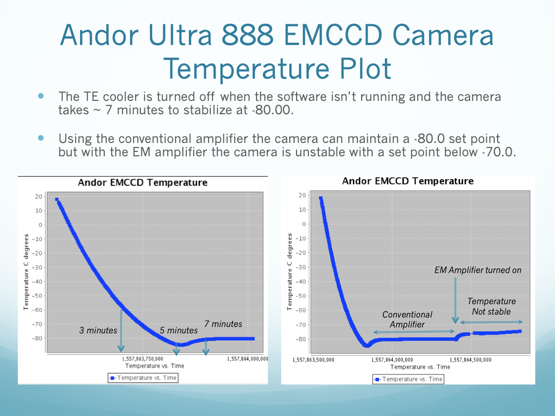
- The camera's thermo-electric cooler is automatically turned off when the software isn't running. Be aware that the camera doesn't automatically reach operating temperature when the software starts and you may need to wait a few minutes for the temperature to stabilize before taking science images.
Camera Operating Temperature
Once the camera software is started and initialized the camera must cool down to the setpoint temperature before science images can be reliably taken. Tasks such as telescope focusing and establishment of point can be carried out during this period. The only reason to wait for the temperature to stabilize before observing science frames (including calibrations) is to minize the dark current and to have constant temperatures during operation. The camera cools from ambient temperature to the setpoint in approximately 5 minutes. The thermoelectric cooler is automatically turned off whenever the software is not running. Obviously the time required to reach the setpoint is determined by the setpoint value. For setpoints equal to −60.00 the camera takes approximately 3.0 minutes but the default setpoint is −80.0 and the camera typically takes 5 minutes to reach −80. The camera temperature will overshoot the setpoint initially by about 5 degrees and will then warm back up to −80.0 in around 7 minutes.
Unfortunately, the Andor Ultra 888 cannot maintain a −80.0 set point temperature when the EM amplifier is in use. When the EM amplifier is selected the temperature will go out of control if the setpoint is −80.0. Under even extremely fast imaging with the EM amplifier the camera can normally operate at a constant temperature of −70.0 degrees. Observers are counseled to watch the temperature during extended runs of fast imaging since ambient conditions (i.e high summer) can make it difficult to maintain stable temperature below −70.0 and they may need to increase the setpoint to −60.0 to continue stable operations.
Camera temperature.
5.e. Miscellaneous Information
- The following information about the camera and software is displayed at the bottom of the ROI tab.
- Andor SDK version (e.g. 2.102.30034.0)
- Controller ID (e.g. USB)
- Camera Serial Number (e.g. sn = 10343)
6. Specialized Tools
6.a. CHIMERA Image Displays
The CHIMERA software can display images using three separate mechanisms:
- a real-time image control that always displays the most current image
- a summed image control that displays the cummulatively summed image as the FITS cube is being acquired and
- a mechanism to automatically display the image in DS9. The real-time (RTD) and summed image displays are accessed from the "Observing Controls" menu in the upper left corner of the instrument control panel.
Each of the FITS image displays have a common basic design and support pan and zoom capabilites as well as mouse driven coordinate (both image and wcs coordinates) and data value displays. The real-time display supports a simply brightness and contrast contrall accesible from the "Image" menu at the top of the control. The summed image display supports a more specialized and sophisticated brightness and contrast control that is required for make the constantly changing range of values in the image more amenable to display.

Image display controls.
6.b. Target Acquisition and Placement
The CHIMERA image cubes are populated with a set of preliminary WCS keywords. The image displays use the WCS information to map pixel coordinates to the RA and Dec in the image. The image displays integrate the WCS coordinates with the mouse using two separate cursors; the target and bullseye cursors. Observers can use these two cursors to automatically calculate the telescope move required to move the "target" object to the "bullseye" location in the image. Use the following steps to place an object at a particular location in the image.
- Start the camera in "Targeting" mode so that the image is "live."
- Place the mouse on the image and then right click to bring up the cursor menu (alternately select the Target Cursor in the Mouse Control combobox)
- Select the Target Cursor and then place this cursor on the object you wish to move in the image.
- Now select the Bullseye Cursor and place this cursor at the position where you want to move the object.
- Note that the distance in arcseconds between the target and bulleye cursor positions in both RA and Dec are now displayed beneath the Move Target to Bullseye button. It's good practice to verify that these numbers make sense before trying to actually move the telescope.
- Press the Move Target to Bullseye button. This sends the command to the TCS to move the object at the target position to the bullseye position. The progress of the motion is depicted in the telescope motion progress bar.
- Since you are in targeting mode with the camera "live" you should see the object move from the target position to the bullseye position.
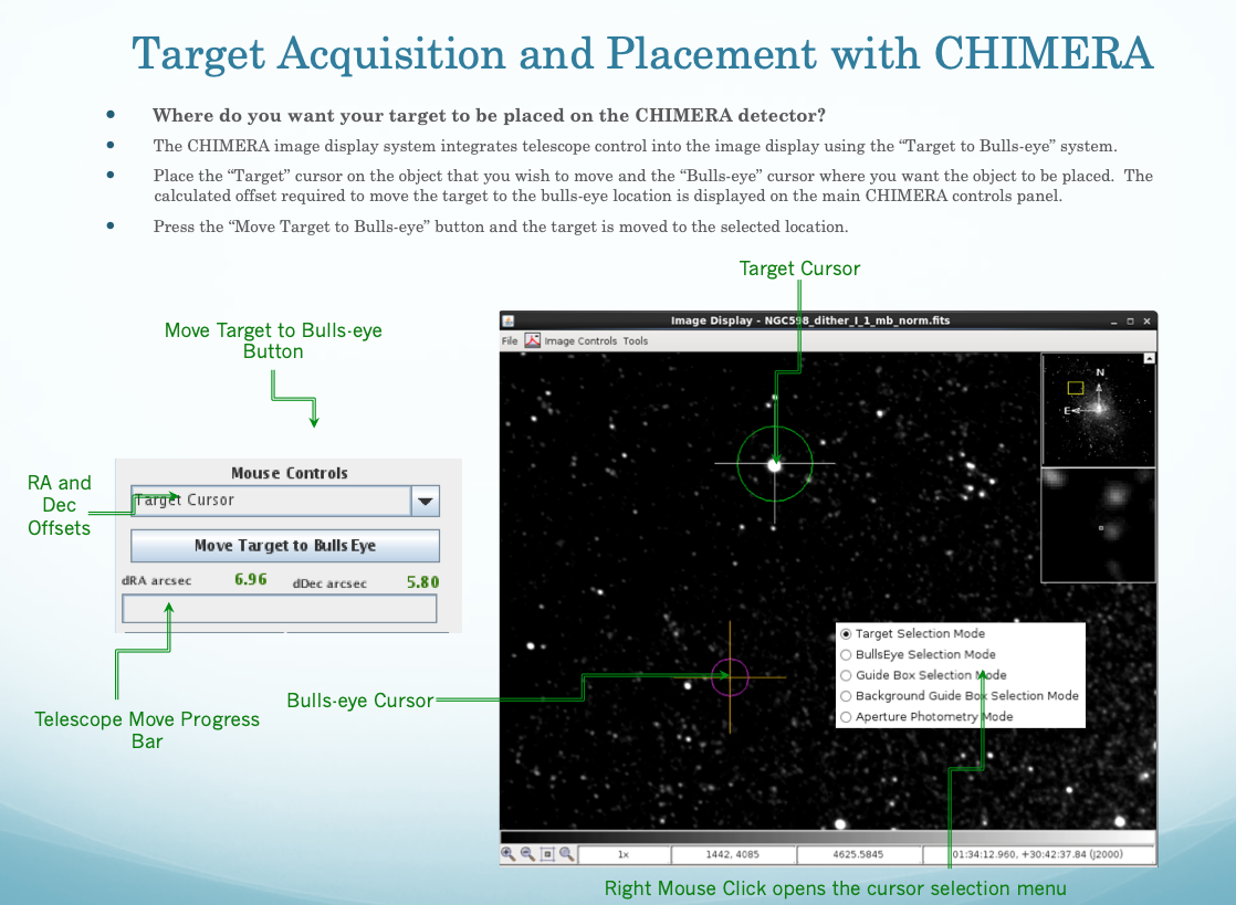
Target to bullseye.
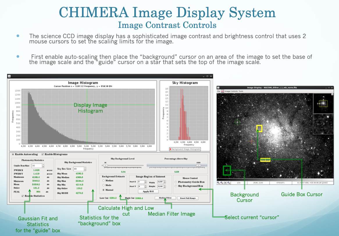
The summed image display presents the cummulative sum of all the images in a FITS cube as the cube is being observed. The observer can configure the summed image display to reset after the completion of each cube or to simply keep summing the image from one FITS cube to the next. Controls are also available to clear the summed image memory to reset the image. When you are looking at an image whose count levels are continuously changing as each new image is added to the sum it can be hard to keep the contrast and brightness from just turning the entire image white. A specialized image contrast and brightness control designed specifically for continuously summed images is available for the summed image display. The summed image contrast control uses the guide box and background cursors to set the upper and lower limits of the stretch. The typical way this control works is to place the background cursor box in a portion of the image that has few or no stars. The background cursor box sets the lower bounds of the image stretch. The guide box cursor is then used to set the upper end of the stretch scale. Experience has shown that placing the guide box cursor on a very faint star achieves the optimum stretch, bringing out the structure of the background and making even very dim objects visible in the image.
The summed image display contrast controls provide a considerable amount of information about the currently displayed image. For the object within the guide box the control displays the FWHM in both X and Y as well as the maximum, minimum, mean, standard deviation of fitted peak height. The control also provides a variety of metrics for the portion of the image in the background box including the mean, median, maximum, minimum, standard deviation and the mode. The background box represents an excellent way to measure the sky background during observation. The upper portion of the contrast and brightness control displays a complete histogram of the currently displayed image (i.e. after setting the upper and lower bounds) and a smaller histogram of the flux in the background box is displayed at the top right. The contrast control is enabled by default but to save processing overhead you can turn off the control by un-selecting the Enable Autoscaling checkbox.
Summed image contrast control.
6.c. CHIMERA Timing
For some observations the timing of each frame is important and this need is addressed by connecting the TTL trigger output of each camera to the systems Meinberg IRIG-B GPS card. The GPS card contains a FIFO buffer that can capture up to 500 trigger events from two separate sources (i.e. CH0 for RED, CH1 for BLUE). Meinberg provides a command line program called mbggpscap that can capture the "fire" TTL output signal produced by the Andor Ultra 888 cameras. The "fire" TTL signal is triggered when the TTL signal drops at the end of an exposure and the GPS card captures this event in the FIFO buffer. The mbggpscap program is then used to monitor the FIFO buffer and consume the "fire" event for each camera. A separate "gps_server" program is started prior to starting the software for either camera and provides a mechanism for separating the event received by each camera. When the CHIMERA software starts it automatically connects to the gps_server program over a TCP/IP connection. If the gps_server program hasn't been started a dialog box will appear giving the observer that choice to retry the connections or to ignore it. The way the system works is that each time a FITS cube is to be observed the camera program sends a command indicating that a new FITS cube is to be created and passes along the name of the FITS image file that will be constructed. The gps_server program then clears the arraylist containing any events associated with the camera and starts to accumulate any new events. When the observation is completed the camera program signals that the observation is complete to the gps_server program that then writes out the timestamp events to a file named the same as the FITS cube but with a .txt extension. If you select the Auto-update FITS timing checkbox at the bottom of the instrument controls panel then a copy of the original FITS cube is created with the GPS timestamps added to the header.
There are 4 different timestamps that document the time of an observation: (1) the UTCSTART header keyword, (2) the start acquistion timestamp in the timing.log file, (3) the first frame arrival timestamp in the timing.log file and (4) the GPS timestamp recorded in the $IMAGE_NAME.txt file where $IMAGE_NAME is the name of the FITS cube file. Let's consider the relative timing and significance of each of these timestamps.
- UCTSTART timestamp - the
UTCSTARTtimestamp is created from the computer system clock during the process of creating the FITS header before the header is written to disk. Analysis of theUTCSTARTtimestamp relative to the other timing measurements indicate that theUTCSTARTtimestamp is measured approximately 283 milliseconds +- 10 milliseconds before the command to start the image acquisition is sent to the camera. Of all the timestamps theUTCSTARTtimestamp is by far the least accurate and really records the time that the FITS header is created rather than when the first image is observed. - The start acquisition timestamp is constructed immediately before the "StartAcquisition" method is called. The "StartAcquisition" method initiates the sequence of observations in the camera and appears to take approximately 20 milliseconds (+- 1 millisecond) to actually begin exposing the CCD. This timestamp is recorded in the timing.log file in the current data directory.
- The first frame arrival timestamp is also recorded in the
timing.logfile and records the time that the camera electronics first indicate that a frame is available for retrieval. The first frame arrival time occurs approximately 116 milliseconds (+- less than 1 millisecond) after the actual exposure has terminated. During this 116 milliseconds the software is polling the camera to determine if an image is available and records the timestamp once it receives the indication that the image is available but before the image is retrieved. - The GPS timestamps recorded in the
$IMAGE_NAME.txtfile or included in the FITS header if the Autoupdate FITS timing checkbox is selected are by far the most accurate timestamps provided by CHIMERA. The Andor Ultra 888 EMCCD camera transmits a TTL signal on the "fire" output line that is routed to the IRIG-B PCIe card. Thembggpscapprogram provided by Meinberg is used to capture the "fire" TTL signal events that corresponds to the end on an exposure. If you know the end time of the first exposure from the GPS capture you can rigorously predict the start and stop time for every exposure in the cube using the kinetic cycle time written in the FITS header with an accuracy and precision of +- <1millisecond. There will always be one GPS timestamp for each frame in the FITS cube and if the header is updated then the timestamp for each frame are included in the header with the keywordT$Nwhen$Nis the image number. There are often more timing events recorded than there are images in the FITS cube however. During observation the software puts the camera into a run until abort mode and records the number of images requested (i.e. the cube size). If the camera is running very fast (i.e. exposure time less than 100 milliseconds) then it's possible that the processing will fall behind a little and 105 frames were taken when only 100 were requested. In such a case the first 100 images will be retrieved and written to the FITS cube and the last 5 images are discarded. In this case however there will still be 105 timestamps in the associated timing file. Considerable testing has been done to assure that the first image timestamp in the timing file always corresponds to the timing for the first image in the FITS cube. Additional timestamps at the end of the observing sequence can be safely ignored.

GPS timing.
The typical observation scenario for CHIMERA is to setup both cameras to acquire one FITS cube after another in a continuous fashion for both channels. For example, we might setup 100 image cubes with 1 second exposure time that are taken continuously one after the other for 5 or 6 hours to observe an exoplanet transit or an eclipsing binary. How much time is taken up between observing two consecutive FITS cubes? The overhead associated with starting a new image cube and/or closing the previous cube turns out to be independent of the observing parameters. In other words, it doesn't matter what the exposure time, number of images or exposure parameters are it always takes approximately 1.6 seconds from the end of light collection in one cube before the first exposure to light in the next cube. This means the you will always have a 1.6 second gap in temporal coverage between FITS cubes. The goal with CHMERA observations is always to maximize the amount of time that the camera is collecting light and minimize the amount of time that is spent setting up the observations. To maximize open shutter efficiency it is normally better to set the number of images per cube to near the maximum (i.e. maximum FITS cube size is 2Gb) to minimize the overhead associated with creating a new cube. This advice is particularly applicable when the exposure time is short (i.e. less than 1 second) since the total time per cube is also short and more overhead is incurred by the number of inidividual FITS cubes observed. On the other hand, if the observing program is using the conventional amplifier and the exposure times are long (i.e. > 30 seconds) then a single cube could take 4 hours to observe. The risk that some event might disrupt the observing during a single 4 hour observation is probably too great and half the night would be lost if a single FITS cube failed for some reason during the observation. As a rule of thumb, try to keep the observing time for an individual cube to less than 15 or 20 minutes.
6.d. Using the Ultrafast Acquisition Mode
The Ultrafast Acquisition Mode is designed to minimize all of the potential overheads that can degrade the open-shutter efficiency of the camera during high speed data acquisition. This mode turns off the image display system and all of the analytical tools (i.e. FWHM centroid calcuations,etc.) that eat up clock-cycles. This mode is only absolutely necessary when you are attempting to use exposure times that are less than 10 milliseconds but you might benefit from this mode with full frame images with exposure times less than 100 milliseconds. When you use this mode you are flying blind and cannot monitor what the camera is seeing. Use this mode only when it's necessary to attain greater than 90% open shutter efficiency with very short exposure times. This mode is engaged by pressing the "Utrafast" button on the main instrument control GUI (not the simplified interface).

The ultrafast observing mode.
6.e. Focusing CHIMERA
Focus the telescope with the RED channel and then adjust the BLUE channel focus using the "Birger" mechanism so that the RED and BLUE channel are parfocal.
Once the mechanisms have been homed the system is ready for on-sky operations. The first task is to focus the telescope and this needs to happen in a particular order. Each of the cameras has a "Birger" focus and aperature control mechanism that can be used to focus the camera. However, first we need to focus the telescope using the RED channel camera before adjusting the BLUE channel focus with the "Birger" mechanism. To focus the telescope you first open the real time Fits Image Display control (from the main menu bar) and then select the Autofocus Control from the Tools menu. When you have an image in the display showing the sky, right mouse click on the image and select the Guide Box Cursor radio button. Once the "Guide Box Cursor" is activated you can select a star near the center of the field that has sufficient signal to noise to make accurate seeing quality measurements. Simply left mouse click on the star and a "Guide Box" will appear around the star. If the tool can fit a Gaussian to the selected star then a cross will appear in the guide box indicating that a fit was possible. Once you've selected a viable star for focus you can turn your attention to the "Autofocus Control". The "Autofocus Control" works by starting below best focus and taking one image at each focus increment (default = 0.1mm) for a set number of images and analyzing the star in the guide box to calculate the FWHM as a function of focus. Typically the number of steps used in the "Autofocus Control" is either 10 or 20 dependenting upon how far from focus the initial image appears to be (default = 10). The "Autofocus Control" calcuates the FWHM in the X and Y directions of the image as a function of telecsope focus.When the seeing is reasonable (i.e. below 3 arc seconds FWHM) the resulting plot will display 2 parabolas that are slightly offset from one another. The software fits a parabola to each data set (i.e. X, Y), determines the point of inflection and calculates the best focus as a point halfway between the inflection points. However, the data is often noisy (i.e. the parabolas are far from perfect) and the calculated value can be misleading; this is particularly true if the data collection isn't symmetric about best focus. Often the best way to determine best focus is simply to look for the minimum in the displayed FWHM vs. telescope focus curves and then manually set the telescope focus to that value. At this point the RED channel has been focused and you need to turn to the BLUE channels adjustment.
Focusing CHIMERA.
Once the RED channel has been focused we then need to refine the BLUE channel focus using the "Birger" focus control mechanism. Start by opening the real time Fits Image Display for the BLUE camera, put the instrument into "Targeting" mode and begin taking images. Once a star field is being displayed you can select a star using the "Guide Box Cursor" as described above and make sure that the Start Measurement button is active. Next, open the PSF Graph button for the real-time display and you should see a graph that displays the current FWHM as a function of time. Now open the Canon CHIMERA focus and aperture control from the main instrument control panel's menu. The "Birger" focus mechanism should already be connected and ready for adjustment (i.e. all the status icon's are green). Now while the camera is running in "Targeting" mode, slowly adjust the "Birger" focus using the offset arrow controls (i.e. these controls move focus up (right ) or down (left)) and observe what happens to the FHWM on the PSF graph. Adjust the focus until you convince yourself that you can identify the focus encoder value that give the smallest FWHM. At this point you have adjusted the focus of the BLUE channel so that its parfocal with the RED channel.
Start by focusing the telescope using the RED channel
- Before you start focusing the RED channel, set the RED channel Birger focus to 9000 so that the BLUE channel will be within adjustment range after focusing the RED channel.
- Open the real-time display window (RTD).
- Right mouse click on the image and select the Guide Box cursor.
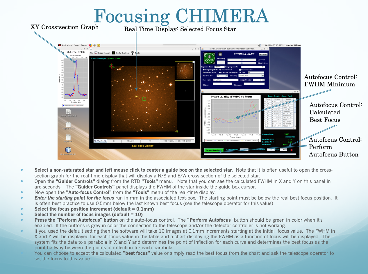
- Select a non-saturated star (preferably near the center of the detector) and left mouse click to place a guide box on the selected star. Note that it is often useful to open the cross-section graph for the real-time display that will display a N/S and E/W cross-section of the selected star.
- Open the Guider Controls dialog from the RTD Tools menu. Note that you can see the calculated FWHM in X and Y on this panel in arc-seconds. The "Guider Controls" panel displays the FWHM of the star inside the guide box cursor.
- Now open the Auto-focus Control from the Tools menu of the real-time display.
- Enter the starting point for the focus run in mm in the associated text-box. The starting point must be below the real best focus position. It is often best practice to use 0.5mm below the last known best focus (see the telescope operator for this value).
- Select the focus position increment (default = 0.1mm).
- Select the number of focus images (default = 10).
- Press the Perform Autofocus button on the auto-focus control. The Perform Autofocus button should be green in color when it's enabled. If the buttons is grey in color the connection to the telescope and/or the detector controller is not working.
- If you used the default setting then the software will take 10 images at 0.1mm increments starting at the initial focus value. The FWHM in X and Y will be displayed for each focus value in the table and a chart displaying the FWHM as a function of focus will be displayed. The system fits the data to a parabola in X and Y and determines the point of inflection for each curve and determines the best focus as the point halfway between the points of inflection for each parabola.
- You can choose to accept the calculated Best Focus value or simply read the best focus from the chart and ask the telescope operator to set the focus to this value.
Adjust the BLUE channel focus using the Birger Focus Control to be parfocal with the RED channel
- Open the RTD on the BLUE channel and place a guide box cursor on an un-saturated star (see above)
- On the "Advanced" Instrument Controls GU, turn on "Start Measurements"
- Display the PSF graph - the FWHM for both the X and Y direction will be displayed like a chart recorder
- Adjust the BLUE channel Birger focus until the FWHM in X and Y are at a minimum and comparable to one another in value
- At this point the BLUE channel camera is parfocal with the RED channel. If the RED channel is at best focus then the entire instrument is in focus.
6.f. Guiding with CHIMERA
Applying a telescope position correction during observing (guiding) takes time. Unfortunately, this is a fundamental limitation of the interaction between analyzing an image and applying a position correction to the telescope. Because guiding does in fact take some time it can affect the open shutter efficiency that an observer experiences when observing. To guide effectively without degrading the open shutter efficiency of your observations you need to consider just how fast the P200 telescope drifts. The typical position drift of the P200 telescope is approximately 1 arcsecond every 15 minutes. This value can vary depending upon the telescope orientation but in general it varies from 1 to 3 arcseconds every 15 minutes. The drift is small and a stars centroid will move 1 pixel in a little over 4 minutes. To keep an object on the same pixel during a prolonged observation (e.g. a light curve) it's not necessary to have a high bandwidth. Having a high bandwidth (i.e. making frequent position corrections) is often a good thing. However, with the P200 telescope it's not necessary.
There are really two cases that have to be considered:
- Correction using every image linked to the real-time display.
- Correction using the sum of a FITS cube linked to the summed image display
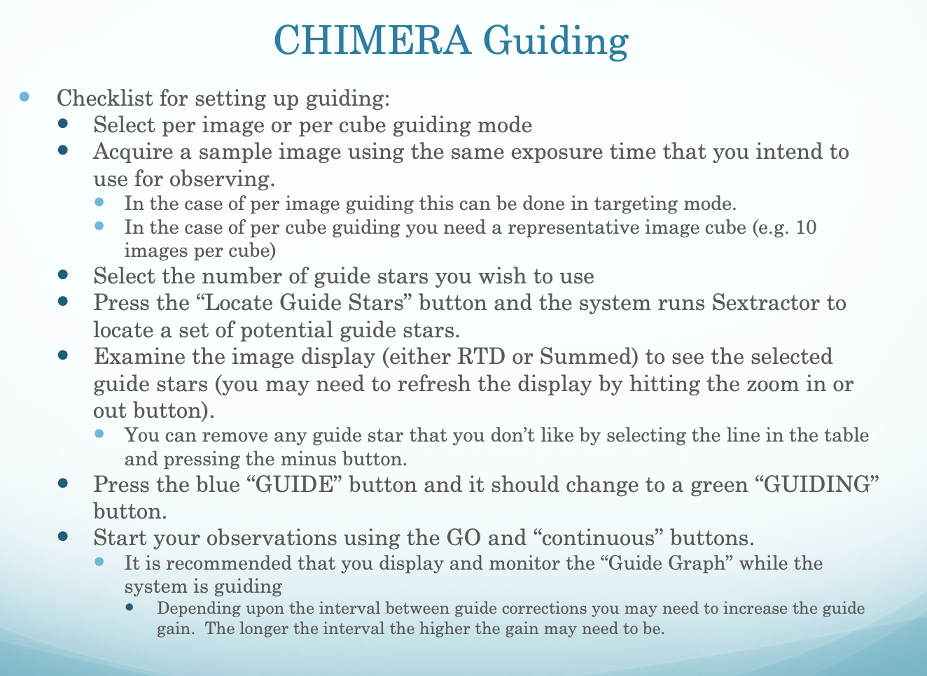
CHIMERA guiding checklist.
It's important to consider how long it takes to make a position correction (i.e. from 200 to 500 milliseconds) compared to the exposure time. Obviously if you are observing with a 100 millisecond exposure time and you spend between 200 and 500 milliseconds to correct the position for each image; your open shutter efficiency is going to be terrible. The cutoff between reasonably high open shutter efficiency and guiding occurs somewhere around a 3 second exposure and per image guiding should be used in general for exposure time greater than or equal to 3 seconds.
The other case is a little more unusual; guiding on the sum of a FITS cube. When you are observing with very short exposure times (particularly less than 1 second) it is impossible to make a guide correction on each individual frame without seriously degrading the open shutter efficiency. The CHIMERA software can automatically construct a summed image of an entire FITS cube and use this image as the basis for a guide correction. The frequency of the guide correction is then linked to the number of images in the FITS cube and the total exposure time represented by the cube. Typically you want to make guide corrections at least every 5 minutes (i.e. the total time to acquire a FITS cube) so that the correction does not have to move the centroid more than ~1 pixel.
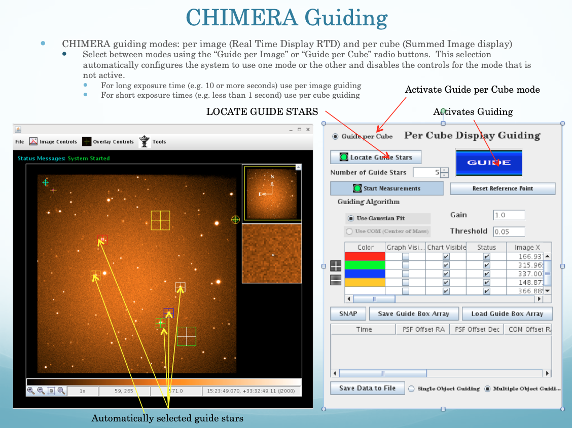
CHIMERA guiding.
7. Conclusions
CHIMERA is a powerful instrument and it can be difficult to quickly learn all of its capabilities. However, the most fundamental task of the instrument, acquiring near simultaneous FITS cubes in both the RED and BLUE channels, is rather simple. Once the instrument has been setup and readied for observing (i.e. mechanisms homed, gps time stamping started, focus acquired) you simply need to specify the following parameters:
- Exposure time
- Conventional or EM gain amplifier (and EM gain if using the EM amplifier)
- Do you want to use frame transfer?
- Horizontal Readout Rate
- Number of images per FITS cube
- Image Name (i.e. if different from the defaul)
Once you have specified these parameters you can turn on continuous mode, put the instrument into "SCIENCE" operations mode and start taking images by pressing the GO button on both cameras. The instrument will then start collecting FITS image cubes one after the other until you turn the Continuous button off. This is by far the easiest way to collect the images required to make a light curve; all the additional controls are unnecessary if this is all you want to do. When you're observing pay attention to the calculated open shutter efficiency which should be greater than 90% if you've choosen your parameters wisely.
Questions? We've answered many common observing and operations questions in our observer FAQ page.
Please share your feedback on this page or any other Palomar topic at the
COO Feedback portal.
Chimera Manual / v 1.0.0
Last updated: 26 February 2020 JM
|
|
|