
|
|

|
Triple Spectrograph (TSpec) Cookbook
View the original cookbook.
- Spectrograph
- Guider
- Object data
- Exposure times
- System response
- Standard stars
- Continuum sensitivity plots
- Flexure information
Contents
1. Spectrograph
1.a. Basics
- In the near-infrared the OH lines from the sky are strong and variable, and in the K-band thermal emission is seen from the telescope and sky. There are also a significant number of bad pixels in the array. As such it would be a good idea to take spectra at different positions along the slit.
- There can also be some flexure (~0.5″ / 1 pix) when going from vertical to horizontal with the spectrograph, so even if the OH lines didn't vary you may see poor subtraction of the lines.
- You can also get a quick look at your data by taking the difference of two different positions along the slit (with the provisos above). For short integrations (~30 seconds) a simple difference is likely to work well.
1.b. Setup
- The data directory path is set by the support astronomer, and can be seen on the spectrograph GUI. See below #5 in the Spectrograph GUI section.
- Select starting file numbers for the night (e.g. 1000 for night 1, 2000 for night 2, etc).
- Select desired number of Fowler samples.
- The integration time will be set appropriately for each object.
1.c. Calibration Data
- Dome flats:
- Take with the dome dark, mirror cover open.
- High lamp: t = 30 seconds, 10 images to average
- Lamp off: t = 30 seconds, 10 images to average
- Calibrators:
- Choose an Elias standard or one from the supplied list of A0V stars
- For future reference place a marker box at the location of the star before moving it onto the slit (this will help with acquiring sources later)
- For Elias stars, t = 30 works for most
- Take spectra at 5 positions along the slit (you can use the Take Seq button in the Guider window).
1.d. Spectrograph GUI
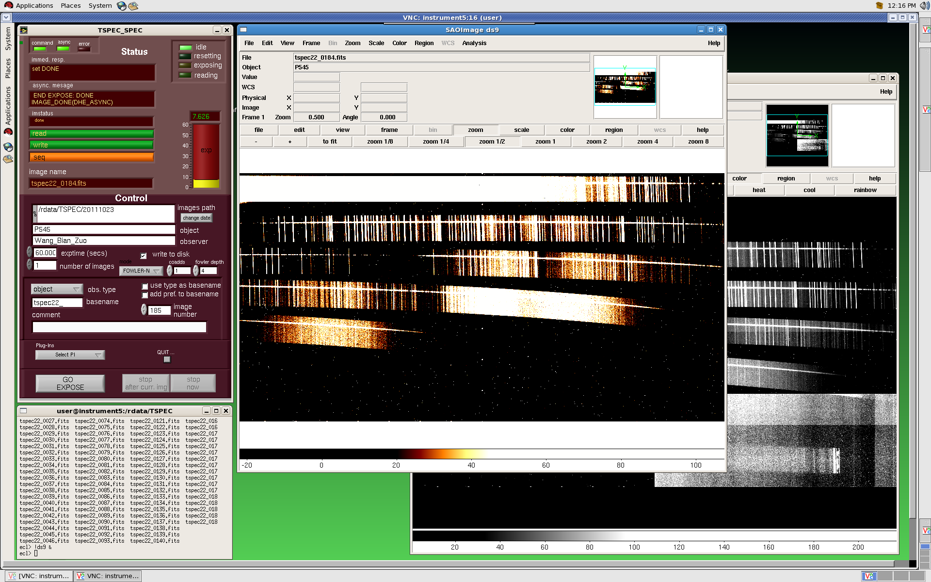
Desktop 1.
- Above is a snap shot of the spectrograph control GUI, a DS9 session, and an IRAF window, as they typically appear on one of the dual displays on the workstation running TSPEC in the 200-inch control room. For this document it will be assumed that the observer knows about DS9 and IRAF. If you need help with DS9 or IRAF, talk to the instrument support engineer in the afternoon when you get to Palomar.
- The window in the upper left is the camera control GUI. This GUI is a LabVIEW + C code based architecture we call ARCVIEW, that runs many of the Palomar public instruments.
- The lighter colored upper half of the GUI, titled Status, is purely informational, and not controllable.
- The darker lower half of the GUI, titled Control, is what the observer uses to control the spectrograph camera. The following bullets in this section detail the Control section features from top to bottom.
- The image path is set automatically when the GUI is started, or when
the user pushes the change date button next to the image path.
This automatically creates a new directory in
/rdata/TSPEC/for the current UT date. - The exptime window is of course the exposure time of the next image in seconds. Below exptime is the window which selects the number of consecutive images that will be taken at the selected exposure time when GO EXPOSE is pressed.
- The write to disk selector should always be selected. The observer must save the image to disk
in order to
eventually see it on DS9 with the
displaycommand in the IRAF window. - The number of coadds and Fowlers can be selected just below the write to disk selector. If you are unfamiliar with coadds or Fowlers, talk to instrument support.
- The next section deals with more exposure information. The pull down
that currently reads
noneselects image type information (object, dark, flat, etc.) which goes in the header. basename is the image file prefix. use type as basename selects the image type from the image type pull down and makes that the image prefix. Do not use add pref. to basename, since it can crash the GUI. - comment adds comment information into the FITS header.
- The Plug-Ins pull down selects some sub-vi windows (temp, ROI, header, etc.) that don’t have too much application to this instrument.
- QUIT is a very important button. Pressing QUIT
brings up the hidden QUIT button. QUIT is the nice
way to shut down the camera control GUI. Use QUIT if the GUI
seems hung, and when the control GUI disappears, re-start with the
TSPEC_SPECicon found in theTSPECfolder on the VNC desktop. Instrument support will show you how to do this. - The last three buttons at the bottom of the control GUI are GO EXPOSE which starts an exposure (or exposure sequence), stop after current image which cleanly stops a sequence of images when the current image is finished reading out, and stop now which stops an exposure (and exposure sequence) by reading out the chip. These two stop buttons are preferred to put a clean halt to things.

Spectrograph control GUI.
2. Guider
2.a. Guider GUI

Desktop 2.
- Above is a screen shot of the guider VNC window as it will appear on one of the monitors on the workstation on which you will be running Tspec.
- Most of your time observing will be spent in this window. The guider GUIs controls the dithering sequence, the guiding, the images the guider saves, AND IT REMOTELY CONTROLS THE SPECTROGRAPH (taking images during the dithering sequence).
- In the upper right is a green window that looks very much like the spectrograph camera control GUI. This is in fact the LabVIEW/ARCview camera control GUI for the guider camera. It is laid out just like the spectrograph GUI. Status information in the top half, and camera controls on the bottom half.
- As with the spectrograph, the status indicators are self explanatory. Starting from the top of the control half, there are the object and comment windows in which the observers can enter information into the IRAF headers.
- The exptime and num. of images windows are just like those on the spectrograph.
- The cont_read control is for the guider in continuous read mode. This mode is usually used for guiding. Clicking on this control deselects continuous read, and the write to disk selection appears. When write to disk is selected, the bottom of the control GUI expands to include the following: image path, observer (FITS header entry), image base name, image number, and the obs. type pull down menu that selects the image type for the FITS header. This write to disk section acts just like the same windows in the spectrograph GUI, except this information is applied to the saved guider images.
- Below the the write to disk selector is a write last button. Press this button and the GUI will save the image currently in the Guider buffer even though write to disk is not selected.
- Just below write last is the small QUIT button that brings up the QUIT button. QUIT cleanly brings down the camera control GUI, which is useful if the camera (PCI card) locks up.
- The Select PI menu has two selections; one is headers that brings up a FITS header vi, in which the observer can add FITS header information. The other selection is sguide which is the slow guider display window to the left of the camera control GUI. Since this window comes up at start up, the observer should never need to select sguide.

Guider control GUI.
2.b. The Slow Guider Display Window
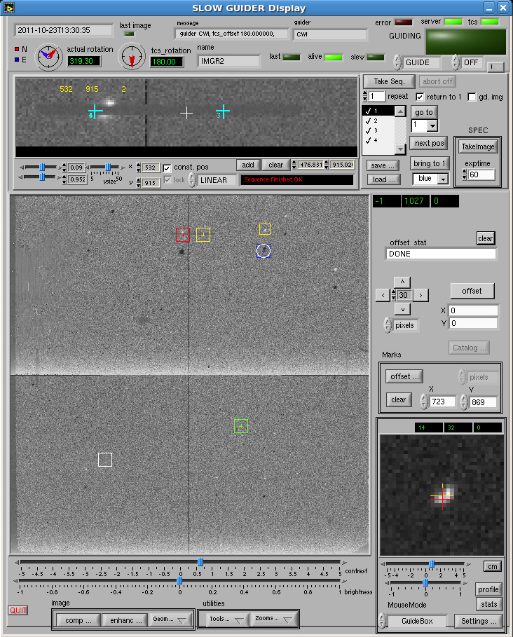
Slow guider display.
- The window to the left of the Control GUI is the imager, the dithering tool, the remote spectrograph control, and the launching pad for many pop up GUIs.
- The image seen in the snap shot above shows the guider reflective surface. At the top can be seen the 1″ × 30″ slit, which in this snap shot has a small yellow square sitting on the right side of the slit, and a small red square on the left. In the bottom, left, and right, appear other slits. In the Palomar version of Tspec, these three other slits are not used.
- Above the main image is a zoomed-in image of the slit. This is where the observer places the slit dither marks. Various controls for the placing of marks are located below the zoomed-in slit image.
- To the right of the zoomed-in slit imager are the dithering sequence and remote spectrograph setup and controls.
- Above the zoomed-in imager and dithering controls, is the guider control and telescope status indicators. Guiding is relatively easy; just put the yellow guide box on a star and toggle off to on. As the target is dithered across the slit, the software moves the guide box the same distance to keep the guide star centered in the guide box.
- tcs_rotation refers to the Cass ring rotation. The actual rotation is the chip orientation on sky. The Cass ring and the chip orientation are offset. More on ths below.
- To the right of the main image display is a smaller display that shows the image inside the guider box. There are some contrast controls below this display. On the screen shot above there is a sub-vi to the right of the guider display that is a plot of the intensity profile of the pixels inside the guider box. The actual guider box in the image can be moved and resized with mouse drags. Click and drag to move the box, and click and drag the lower left corner of the box to resize it.
- An important selector in the guider display area is the MouseMode selector. With this you can measure distances, add fiducial marks, and manipulate the guider box.
- Above the guider display area are some controls for the fiducial markers, and offset controls.
- And finally there is a line of pull down menus at the bottom of the main image display window. These selections lead to a vast number of controls and displays. There is an auto contrast sub-vi, an automated focus sub-vi, there are zoom displays for fiducial marks, various one-D plotting tools, image subtraction, and more. See Instrument Support for a tour of these features when you arrive.
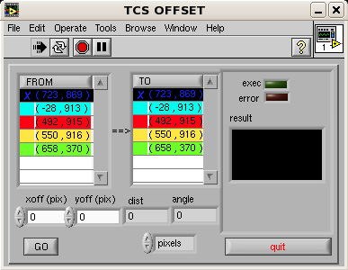
TCS offset.
Slit and Cass Ring Rotation
- The slit and cass ring indicators on the top of the slow guider window can cause some confusion with regards to actual slit orientation on sky.
- The left indicator shows the guider chip orientation on sky. The right indicator shows the tcs ring angle.
- When the ring angle is at 139.32, the Tspec guider is at 0, where 0 is North up and East left.
- Moving to a desired slit angle is confusing because the slit software rotates in an opposite sense to the TCS rotation. The following is a table which shows the values for the four cardinal directions.
| Tspec on sky actual rotation | tcs ring angle tcs_rotation | North & East |
|---|---|---|
| 0.0 | 139.32 | N-up & E-left |
| 90.00 | 49.32 | N-left & E-down |
| 180.00 | 319.32 | N-down & E-right |
| 270.00 | 229.32 | N-right & E-up |
| The slit is East/West when Tspec on sky is North-up & East-left. | ||
2.c. TCS Display
The TCS status display has been modified to show instrument position angle. The convention used is:
| Inst Angle | Slit Position |
|---|---|
| 0.0 | N-left & E-down |
| 90.00 | N-up & E-left |
| 180.00 | N-right & E-up |
| 270.00 | N-down & E-right |
2.d. Guiding Settings
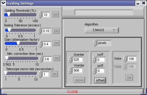
Guiding settings.
This dialog box is called by pressing the Settings button on the Guider area (bottom right corner) of the Guider GUI.
Settings definitions:
Guiding Threshold: Sets the threshold required for the guider to assume there is enough signal to guide. If 5 % of the pixels inside the box area have at least a _threshold_ % value of the peak, then the correction will be sent.Otherwise it will be rejected and an error message will appear on the messages area of the main window ("-34 NO SIGNAL"). Also the "last" LED will be turned off.
Seeing Tolerance: Any correction with a value < Seeing_Tolerance will NOT be sent, assuming they are variation due to seeing and not real corrections.
Gain: This is the "attenuation factor" applied to the calculated correction.This number must be adjusted to avoid overshoot or oscillation on the telescope.
Min Correction time: Sets the minimum rate for the corrections, in seconds. Any correction calculated before _min_ seconds will not be sent.
Telescope Move Rate: Sets the speed at which the telescope will move when a correction is sent (in arcsecs/sec).
Algorithm: Defines which algorithm will be used for the guiding process: CMASS (Center of Mass) or QUAD (four quadrant weighting). CMASS is the algorithm used by default.
Xcenter/Ycenter: Sets a specific position (pixel-precision) for the center of the guide box. When the box is moved with the mouse this value gets updated and vice/versa.
Xoff/Yoff: Sends an offset for the guide box. The offset can be specified in pixels or in arcsecs. If arcsecs are used, Xoff and Yoff become RA and DEC.
Xsize: Sets the size of the guidebox at pixel-precision. This can be specified in arcsecs or pixels.
3. Object Data
- Set up dither positions along the slit:
- It is recommended that you take data in at least two different positions along the slit. For point sources you may want to do more (e.g. 4-5 positions or so) for good removal of bad pixels and sky.
- There is a check box below the slit zoom window which causes the markers to be confined along the slit. It is suggested you use this feature unless you have some special needs.
- Acquire object in guide field. Note: the default position (telescope pointing) should be off the slit.
- Place a marker box on source and use cm button in the corresponding zoom box to center the box on the source.
- Place the guide box over a star that will be in the field when the source is moved onto the slit. Use cm button in the guide box to center the guide star.
- Turn the guider on.
- Select the marker box with the object (e.g. green) and use the bring to 1 button to place it on the slit in position 1.
- Check to make sure your source is on slit position 1 and the guide box is centered well.
- Select the integration time you want for the spectrograph. Note: the value in the Guider window will override the spectrograph value if you use a Take Seq or Take Spec command.
- Use Take Spec or Take Seq command to start taking data.
- Sometimes you want to take a spectrum first before starting a sequence to make sure everything is okay. You can then go to the next position by using the Goto button.
- Note: if you have the gdr img box checked, each time you take a spectrum from the guider window, a guider image will also be taken.
4. Exposure Times
The shortest exposure time is about 4 seconds. There are three possible limits to the maximum exposure time: source saturation, saturation in the K-band and saturation of OH lines. The plot below shows the background measured by TripleSpec near zenith on 16-Feb-2008 (ambient temperature ~ 0° C). Using a saturation level of 28,000 DN, the maximum integration time is approximately 2400 or 1200 seconds for saturation to start occurring in the H and K-band respectively.
The longest integration times we have done on sky thus far are 600 seconds. With a dark current of 0.085 e−/sec and a read noise of 3.5 e− (w/ Fowler sampling), then the noise due to the dark current will equal the read noise in ~ 144 seconds. The inter-OH continuum is difficult to measure but appears to be ~0.1-0.8 e−/s over the J and H-band. This implies that 300 seconds should be sufficient to overcome the read noise. (Note: this result is preliminary.)
5. System Response
Plot of sky + telescope emission for TripleSpec in units of DN/sec taken on February 16, 2008.

Plot of sky DN/sec per column for a 10th mag A0V star.
S/N ratio per column for an m = 15 (A0V type) source. Coadding across a resolution element (3 pixels) will decrease the number of coadds by a factor of 3 or (for fixed number of coadds increase the S/N by a factor of √3. No differencing noise is included.
Same as above but for m = 17.
Same as above but for m = 18.
Same as above but for m = 19
The response (integrated across a column) to at 10th magnitude star is given in the second plot. This can be used for scaling to other magnitudes.
6. Standard Stars
These are a subset of the Elias standards (A-stars). Typical integration times will be 30 seconds. They will be saturated in the guider field. A K-star (or model profile) will be needed to remove the H recombination lines. Additional calibrators can be found via the usual searches on-line.
Name RA (1950) Dec (1950) J H K
HD 225023 00 00 11.8 35 32 14 7.065 6.985 6.96
HD 1160 00 13 23.1 03 58 24 7.055 7.045 7.04
HD 3029 00 31 02.3 20 09 30 7.25 7.12 7.09
HD 18881 03 00 20.5 38 12 53 7.125 7.13 7.14
HD 22686 03 36 18.7 02 36 07 7.195 7.19 7.185
HD 40335 05 55 37.6 01 51 09 6.54 6.47 6.45
HD 44612 06 21 09.7 43 34 35 7.06 7.035 7.04
HD 77281 08 59 05.4 -01 16 45 7.105 7.05 7.03
HD 84800 09 45 35.9 43 53 56 7.56 7.53 7.53
HD 105601 12 06 56.1 38 54 39 6.81 6.715 6.685
HD 106965 12 15 24.0 01 51 10 7.375 7.335 7.315
HD 129653 14 40 38.2 36 58 07 6.98 6.94 6.92
HD 129655 14 41 11.0 -02 17 38 6.815 6.72 6.69
HD 136754 15 19 24.3 24 31 19 7.15 7.13 7.135
HD 161903 17 45 43.3 -01 47 34 7.17 7.055 7.02
HD 162208 17 46 20.7 39 59 40 7.215 7.145 7.11
HD 201941 21 10 13.6 02 26 12 6.7 6.64 6.625
HD 203856 21 21 37.1 39 48 12 6.925 6.88 6.86
7. Continuum Sensitivity Plots
The figures on the right are plots of estimated S/N ratio for an "A0V" star at various magnitudes. These are computed per column so that averaging across a resolution element improves the signal-to-noise ratio by a factor of √3. The estimates are based on calibrator and sky measurements taken in February 2008. The ambient air temperature was ~ 0°C.
Note: An increase in noise due to subtraction of two spectra is NOT included. Whether this is done or not depends on the final reduction technique. If a simple difference of spectra taken at two positions in the slit to remove background and bad pixels then the signal-to-noise ratio will decrease by a factor of √2.
Assumptions:
- Read Noise 3.5 e− (16 samples)
- No. Pixels in extraction: 4
- Fraction of flux in extraction: 0.7
- Spectra not subtracted: no √2 loss due to differencing
- Spectra are not averaged no √3 improvement in S/N or over a resolution element factor of 3 reduction in time (or coadds)
The plot label gives the magnitude, exposure time for each image and the number of coadds (ncoadds). Obviously, the S/N will improve by √ncoadds.
8. Flexure Information
The spectrograph will flex on average about 1/2 pixel. The engineering team did an experiment where they spun the cass cage at 45° zenith angle, and the average flex was 1/2 pixel. They estimate the maximum as 1.5 pixels, considering that some observers will push the telescope over to 60+° zenith angle.
| Wavelength Ranges for each Order (µm) | |
|---|---|
| Order 3: | 2.4644498 to 1.8760142 ± 0.00014177590 |
| Order 4: | 1.8501315 to 1.4103792 ± 0.00010556104 |
| Order 5: | 1.4835071 to 1.1297587 ± 0.000084883749 |
| Order 6: | 1.2379470 to 0.94296033 ± 0.0000654381 |
| Order 7: | 1.0629230 to 0.80778160 ± 0.000060547528 |
| Where the ± is the wavelength amount of 1/2 pixels. You can multiply up for 1.5, if that's the better number. | |
Note that the sensitivity of TSPEC drops off significantly short of 1 µm, so the observers shouldn't get the impression they can get 0.8 µm with TSPEC.
Questions? We've answered many common observing and operations questions in our observer FAQ page.
Please share your feedback on this page or any other Palomar topic at the
COO Feedback portal.
TripleSpec Cookbook / v 2.1.1
Last updated: 31 March 2019 CMH/ACM
|
|
|