1. Install the Anaconda suite, which has all of the packages they will need in Python for astronomy and machine learning.
Mac: https://docs.anaconda.com/anaconda/install/mac-os/ Windows: https://docs.anaconda.com/anaconda/install/windows/ Linux: https://docs.anaconda.com/anaconda/install/linux/
2. Skim through the following webpages. They do not have to devote more than 30 mins-1 hour to looking through them. This is just so that the terms I introduce in Friday won’t be completely alien to them: Intro to Python | Intro to NumPy | Plotting
Intro to Python (presentation)
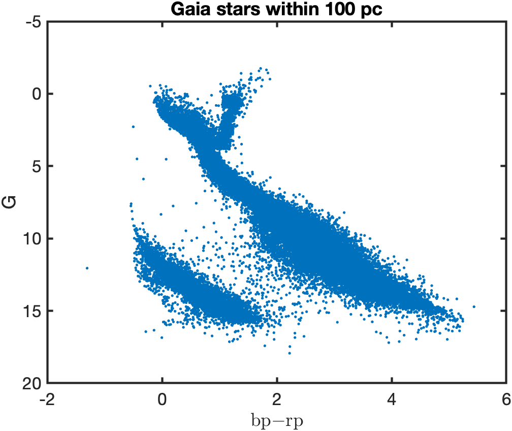
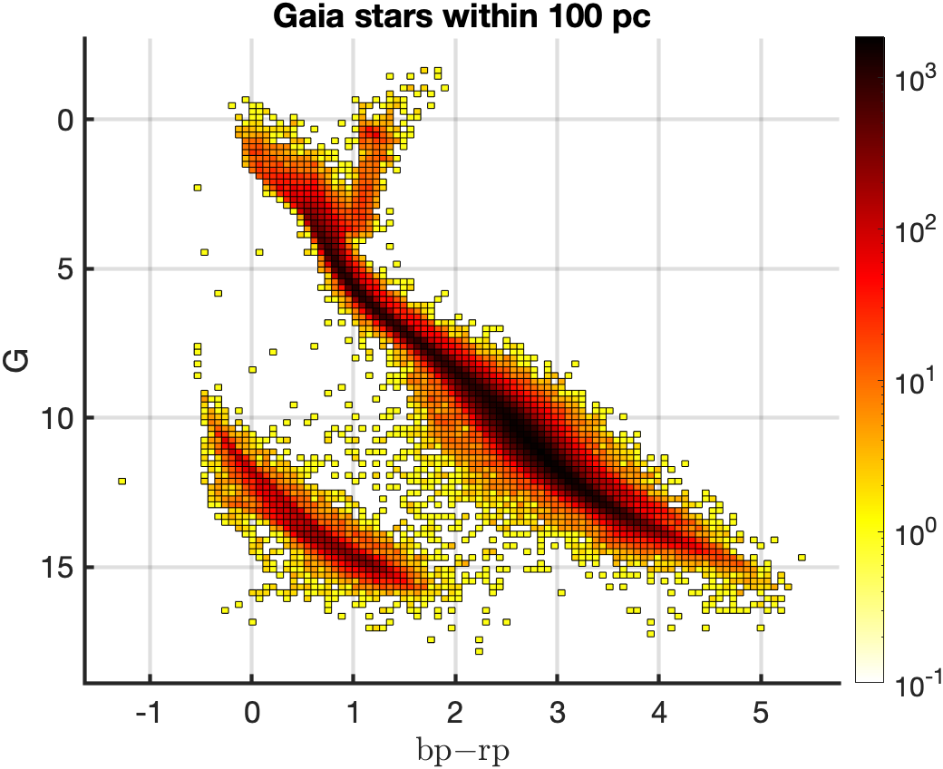
Exercise: Plot the color (bp-rp) magnitude (G) diagram for stars within 100 parsecs. The data file is here
I have plotted the HR diagram in two ways: Figure 1 (each star is a dot) and Figur 2 (contour diagram with logarithmic scale). There is considerable regularity in the stars!
Classwork: Fold RR Lyarea light curves. Instructions can be found here
In this class we reviewed period folding homework. I then talked about standard deviation, variance, Gaussian variates and propagation of errors Next we discussed the concept of "3-sigma" and and "6-sigma" and concluded that the signa-to-noise ratio is a measure of confidence of a measurement. We concluded with a discussion of "optimal" addition of two measurements which led us to the concept of weighted" average and matched filtering. Interested students would benefit from reading Chapter 8 and an ambitious student may wish to also read Chapter 5 of my notes.
The Fourier transform is one of the most basic tool of time series analysis.
On a lighter note please read this article on naming of stellar variables. I think there is practical wisdom in section A1 and A2.
Tony Rodriguez introduced the Lomb-Scargle method and used Python program to search for periodicity. The data file has three columns: JD, magnitude, magnitude_error.
Please review the Python program. Please run the program and become familiar with it. In the class, you will be asked to undertake FFTs of various other time series (which will teach you about aliasing, sidelobes, window functions).
Windowed oberving. Optical astronomers observe sources at night time. Thus, the data stream is not continuous but is periodic (sidereal day). This "windowed" observing leads to beat frequencies. demonstration. Students repeat this exercise but in python in the class. Jupyter Notebook
A serious researcher (or any sort of quantiative analyst) must learn and become very proficient in Unix. It will allow you to move large mounds of files and undertake massive analyses. First read file and then consult this and then tool chest.
Homework: The ZTF group has machine classified variable stars and made their training set available at URL. The primary Reference: van Roestel et al. (2021). Please skim through the paper. You have access to a "Box" directory. Please see this for description of this directory.
Each of are expected to pick at least three types of stars with one being an RR Lyrae type. For each star, first plot the light curve, plotting the "r" (fid=2) and "g" (fid=1) band light curves separately. Then search for period by using Lomb Scargle. Please write up your work as a report. You will be asked to present your work in the class room. Jupyter Notebook
The deep drilling data sets can be found at the "Box" site. I found a few problematic light curves in the original distribution and so have replaced it with the following lcs.tgz which is a "tar file that has been gzipped". Please first "unzip" it and then "untar it". [In Unix: $ gunzip lcs.tgz | tar xvf - ]. In addition I have supplied file filelist which is a list of the light curve files and numbered. It is useful for batch analysis.
Please undertake batch analysis and explored the data. Example exploratory plots: range (max-min) verus mean, mean versus std, highest lomb-scargle power and corresponding frequency, detection of a spike and so on. I expect each of you to make a presentation.
Students present their first foray.
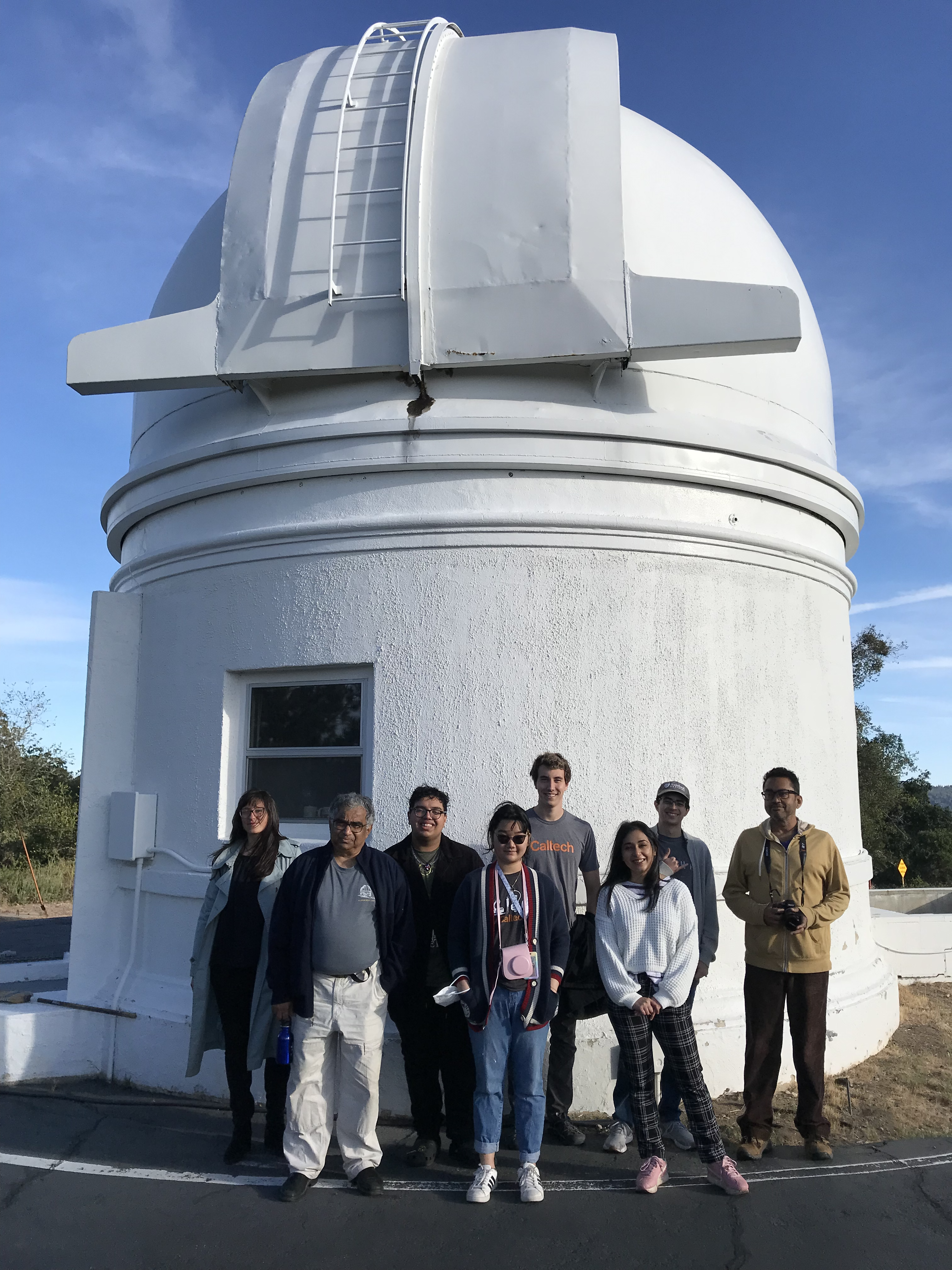
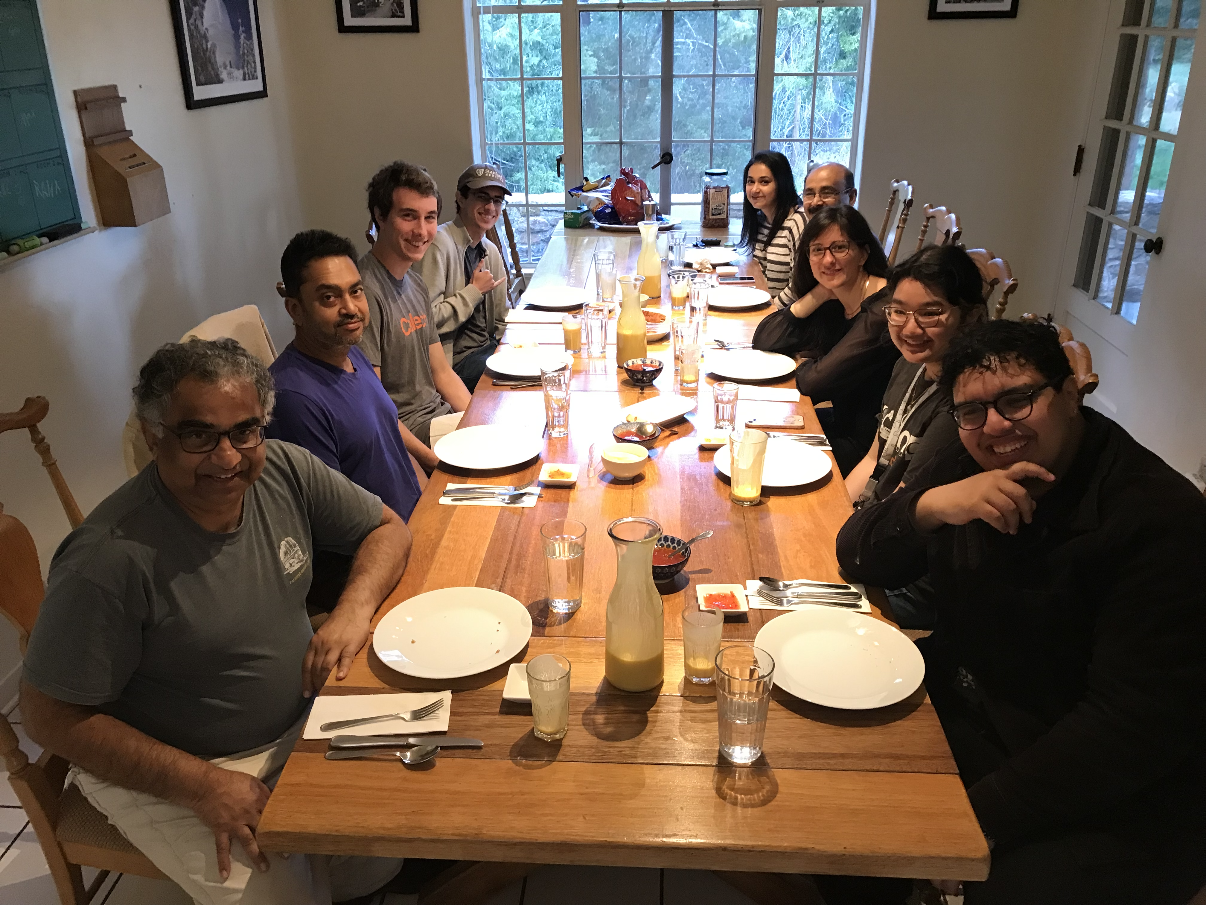
The first picture is P18 dome (established 1935) and used by Zwicky to start his supernova program. We stayed at the historic "Monastery" and Bruce and crew had cooked an amazing dinner.
The talks and the reports constitute the final exam. As such a no-show or a non-submission or an unsatisfactory research (talk/report) will result in F grade.